Analysis of Borrower and Lender Households

Macro Comp Question 1 August 2015

Suppose there are two types of households in the economy. “Borrower” households borrow funds from “lender” households to purchase housing.  Borrower and lender households differ in two ways:  first, only borrowers value housing, while both types value non-durable consumption.  Second, borrowers discount future utility flows more heavily than lenders:  0 < β^B < β^L < 1.   Both borrowing and lending are subject to constraints.

First, consider the problem of borrowers.  Borrowers maximize the expected discounted value of period utility flows with an infinite horizon, where the period utility flow in period t depends on both housing consumption H and non-housing consumption C, as follows:

                                             ∞

(1)Max E  ∑   (β^B)^t [u(C^B_t) + w(H_t)]

                                            t=0

where u(C) and w(H) are increasing flow utility functions.  Housing depreciates at the rate δ, between 0 and 1.  There are no costs of adjustment for housing.  Households enter period t with H_t units of housing, and have (1-δ)H_t units of housing available to retain or sell at the end of the period.  In period t they choose their housing for next period H_t+1. The house price in period t is P_t, which may be time varying and stochastic.  Non-housing consumption is the numeraire, with constant price 1.

In period t, borrowers may borrow D_t+1 ≥ 0 in funds from lender households, at a risk-free interest rate R_t+1, which may be time varying but is known at t.  Borrowing is limited to a fraction of the value of next period’s housing stock by the following inequality constraint:

(2)D_t+1≤ θ P_t H_t+1

Borrower households enter period t with a stock of debt R_tD_t which they must repay to lenders, and receive an endowment of non-durable consumption goods Y_t.  The household’s period budget constraint is given by

(3)                                 C^B_t + P_t H_t+1 =  Y_t + (1 – δ) P_t H_t – R_tD_t + D_t+1

(a) [5 points]:  Identify the minimum set of exogenous and endogenous state variables and the minimum set of control variables, and write down the Bellman Equation for the borrower’s problem.  Don’t forget the inequality constraint (2); let μ_t denote the multiplier on this constraint. 

(b) [20 points]:  Take first order and envelope conditions, and state the complementary slackness condition.  Derive two Euler equations:  one involving only μ_t and values of u'(C) at t and t+1, and the other involving μ_t, values of u'(C) at t and t+1, and w'(H) at t+1. 

Next, consider the problem of lenders.  They also maximize expected discounted utility over an infinite horizon, but their period utility does not include housing:

                                             ∞

(4)Max E  ∑   (β^L)^t u(C^L_t)

                                            t=0

In period t, lenders may give loans L_t+1 ≥ 0 to borrowers at a risk-free interest rate R_t+1.  Lending is limited by the following inequality constraint, where L ≥ 0 is a given parameter:

(5)L_t+1≤ L

Lender households enter period t with a stock of loans R_tL_t for which they receive payment from borrowers, and receive an endowment of non-durable consumption goods X_t.  The lender household’s period budget constraint is given by

(6)                                 C^L_t  =  X_t + R_tL_t  – L_t+1

(c) [5 points] Identify the minimum set of exogenous and endogenous state variables and control variables and write down the lender’s Bellman equation.  Let λ_t denote the multiplier on the inequality constraint (5).

(d) [15 points] Take first order and envelope conditions and state the complementary slackness condition.  Derive the Euler equation for non-durable consumption.    

In equilibrium, housing demand by the borrowers must equal the fixed housing supply H in all periods.  Also, supply and demand for loans must equal:  D_t+1 = L_t+1 in all periods.  In equilibrium, at least one of the inequality constraints (2) and (5) will bind; both may bind.

Important:  for the rest of the problem, assume that the utility function for nondurable consumption for both borrowers and lenders is linear:  u(C) = C. 

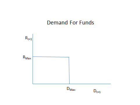
(e) [15 points] Below is a picture of the borrower’s demand curve for funds for this model.  Using the complementary slackness condition and the Euler Equation for nondurable consumption from part (b), explain the shape of this demand curve and express the maximum interest rate R_Max and the maximum quantity of funds D_Max in terms of model parameters and the housing price P. 

(f) [20 points] Using the complementary slackness condition and the Euler Equation from part (d), draw a picture of the lender’s supply curve of funds, expressing any threshold interest rates or quantity of funds in terms of model parameters.  

(g) [20 points] Equilibrium in the market for funds can be expressed graphically by combining the supply and demand curves for funds in a single graph.  Prove that for a given θ, the equilibrium interest rate will equal (1/β^L) when L is sufficiently large, and (1/β^B) when L is sufficiently small.    (Draw one graph for a high value of L and another for a low value of L).