Boiling Point of Polycyclic Aromatic Hydrocarbons

QSPR application on modeling of Boiling Point of Polycyclic Aromatic Hydrocarbons

N. Bouarra^a,b, S. Kherouf^a, A. Bouakkadia^a,c, D.Messadi^a*,

^aLaboratory of Environmental and Food Safety, Department of chemistry, BADJI Mokhtar Annaba University, PB12, 23000, Annaba. Algeria.

^bCenter of Scientific and Technical Research in Physico-Chemical analyzes (CRAPC), BP 384, Siège ex-Pasna Zone Industrielle, Bou-Ismail CP 42004, Tipaza, Algeria.

^cUniversity Abbes LAGHROUR Khenchela – Algeria -BP 1252 Route de Batna Khenchela 40004

Nabil Bouarra Center of scientific and technical research in physicochemical analyzes (CRAPC), Tipaza, Algeria.

Soumaya Kherouf Laboratory of Environmental and Food Safety, Department of chemistry, BADJI Mokhtar Annaba University.

Amel Bouakkadia Laboratory of Environmental and Food Safety, Department of chemistry, BADJI Mokhtar Annaba University.

Djelloul Messadi Laboratory of Environmental and Food Safety, Department of chemistry, BADJI Mokhtar Annaba University.

QSPR application on modeling of Boiling Point of Polycyclic Aromatic Hydrocarbons

Abstract

Physicochemical properties of organic pollutant play an important key role to understand their behavior in environment. However, the information behind the property-behavior phenomena of chemical compounds is less in literature. Therefore, computational methods had to be applied for process optimization.

In the present paper the applicability of the (QSAR), Quantitative structure-property relationship models based on molecular descriptors derived from molecular structures have been developed for the prediction of boiling point using a set of 61 polycyclic aromatic hydrocarbons. For this purpose multiple linear regression was used to construct QSPR model. Best obtained model had following statistical parameters: R²= 99.83, Q²_LOO = 99.8, s =s: 4.5601, F = 11586.1317.

The statistical quality of the prediction results is agree well with the experimental values of this property.

Keywords: polycyclic aromatic hydrocarbons; boiling point; QSPR; applicability domain; external validation; QSARINS

1. Introduction

Polycyclic aromatic hydrocarbons (PAHs) are a group of persistent pollutants widely present in the environment, constituted by hundreds of compounds containing at least two aromatic rings [1]. They are derived from the incomplete combustion of organic matter, due to natural processes such as volcanic eruptions and forest fires, but primarily formed as a result of human activities such as oil spills, burning of fossil fuels, domestic heating systems, transport emissions, and cigarette smoke [2]. Investigations of environmental behaviour of PAHs have attracted considerable attention [3], and due to their toxic, mutagenic and carcinogenic potentials. Particularly benz [a] anthracene, chrysene, dibenz [a,h] anthracene and benzo [a] pyrene [4], are included in the priority list of pollutants of US-EPA[5].

Transport and fate of PAHs in the environment depends, in part, on their physicochemical properties, and their relative distributions between different environmental compartments. One of the most important physical property, used to describe the volatility of a compound (its presence in the atmospheric environment), is the boiling point [6]; defined as the temperature at which the vapor pressure of a pure saturated liquid is 760 mmHg [7]. It is also an indicator for the physical state (e.g., liquid or gas) of an organic compound. Moreover, boiling points can be used to predict or estimate other physical properties [8], such as critical temperatures [9], flash points [10], and enthalpies of vaporization [11]. It is directly related to the chemical structure of the molecule, due to the intermolecular interaction in the liquid and by the difference in the molecular internal partition function in the gas phase and in the liquid at the boiling point [12].

For many PAHs, the values of boiling point are not available in the literature. Their experimental measurement is expensive, consumes a long time and it requires pure compounds. Moreover, the compounds of high molecular weight decompose before reaching their boiling points and require measures under reduced pressure and subsequent correction for atmospheric pressure. Therefore, the direct measurement of the boiling point of the organic compound is laborious [13].QSAR studies have become of major interest in recent years, and especially the QSPR/QSAR models have become a powerful tool for predicting numerous physicochemical propertiesand biological activities of organic compounds. Several studies have modelled boiling point of PAHs. White [14] used simple 1-parameter linear correlation; involving first-order valence molecular connectivity, Todeschini [6] used WHIM descriptors, and Ferreira [5] used the molecular volume (Vol), surface area (SArea), enthalpy of formation(ΔH_f), electron affinity (EA), connectivity indexes (Xe, Xv) and Wiener index (W) by using Partial Least-Squares (PLS) regression. Later, Ribeiro and Ferreira [15] presented a 3 descriptor model using the volume (V), molecular weight (MW) and Randic connectivity index (R) by the means of principal components regression (PCR) and PLS regression method.

In this study, we present a new QSPR model for the prediction of the boiling point of a set of 61 polycyclic aromatic hydrocarbons. Our goal is to develop an accurate, simple, fast, and less expensive method for calculation of boiling point values. The predictive power of resulting model is demonstrated by testing it on unseen data that were not used during model generation; also the Insubria graph was applied to verify the reliability of the predictions of the full model for 57 compounds with unknown data.

2. Material and methods

Developing a QSPR model for boiling point involves several distinct steps, firstly data collection, molecular geometric optimization, descriptor calculation, model development and finally model performance evaluation.

2.1 Data set

The experimental boiling point values of the present work were obtained from [16, 17]. Boiling point range was from 491 to 869 K. A complete list of the compounds names, CAS number and corresponding experimental boiling points is given in the table 1.

2.2 Molecular modeling and descriptors generation

The theoretical molecular descriptors for 61 PAHs were calculated by the following process. Firstly, the molecular structures were pre-optimized by MM+ molecular mechanics force field in HyperChem 6.03 package [18]. The final geometry of the minimum energy conformation was obtained by the semi-empirical method PM3 with a restricted Hartree-Fock level without interaction configuration, applying a standard limit gradient 0.001 Å kcal.mol^-1 as a stopping criterion. Then the final geometries were used as input for the generation of 3224 descriptors of different kinds such as connectivity indices, information indices, topological charge indices, WHIM, geometrical, and GETAWAY descriptors using Dragon software (version 5.5) [19].Other descriptors from HyperChem software were included such as refractivity, total energy, dipole moment, polarizability. Using the corresponding options in Dragon software, we eliminated the descriptors that provide no information (standard deviations less than 0.0001); and then remove high correlated descriptors (r> 0.97), where the variable with the most high cross-correlations with other descriptors was deleted.

2.3 Data splitting

In order to check the predictive capability of the proposed model, before model generation the dataset were split into a training set (~70% of compounds were used for model development), and a prediction set (~30% of compounds were used for external validation). Three different splitting techniques were applied: random splitting, sorted responses plitting and structural similarity ordered by the first axis of Principal Component Analysis (PCA, PC1 score) [20].

2.4 QSPR modeling and validation

The best modeling variables were selected by exploring the statistical quality of all the possible combinations of the available experimental descriptors, by applying multiple linear regression based on ordinary least squares (MLR-OLS) in the QSARINS software (version 2.2) [21]. This ‘variable selection’ procedure generates a ‘population’ of models, ranked according to decreasing R² values. The best models were chosen by using Q² leave-one-out (Q²_LOO) as the optimization value, and taking into account the parsimony principle regarding the complexity of the models, which should be as small as possible. For this reason, only up to three descriptors were included in the QSARs generated in this study. Furthermore, the correlation between the modeling descriptors and the modeled response was checked by the QUIK rule (Q Under Influence of K), to exclude models with high predictor colinearity and exclude chance correlation [22].The best modeling descriptors were selected using all subset procedure of QSARINS software [21, 23]. The search of the best solution was made by maximizing a selected fitness function, in our caseQ²_LOO.

Within the context of REACH, the development of QSPR models is encouraged providing that they respect the 5 driving principles for the validation of QSPR models drawn up by OECD (2007) [22]: 1) a defined endpoint, 2) an unambiguous algorithm, 3) a defined domain of applicability, 4) appropriate measures of goodness-of-fit, robustness and predictive power, 5) a mechanistic interpretation, when it’s possible.

The fourth OECD principle requires suitable measures of performances. Firstly the goodness of the model was reached by verifying the model fitting and the model robustness using respectively the squared correlation coefficient and the cross-validation by the leave-one-out method ().

(1)

(2)

Where is the observed dependent variable (the experimental response), is the calculated value by the model, is the mean value of the dependent variable, n is the number of compounds in the training set, andis the value predicted by the model built without the compound i.

Cross-validation method by the leave-one-out (LOO) is the most known and used method for calculating internal validation. Internal validation techniques are based on iterative data set splitting, i.e. a certain number of molecules are involved in the model calculation (training set), while others(test set) are in turn put aside and used to check the model’s ability to predict them. In LOO the chemicals are put in test set singularly at each iteration.

A stronger internal validation is performed by using the leave-many-out (LMO) procedure. By design, model validation by LMO employs smaller training sets than the LOO procedure and can be repeated many more times due to possibility of larger combinations in leaving many compounds out from the training set The premise being that if a QSPR model has a high average in validation, we can reasonablyconclude that the obtained model is robust[23]. In our case, 30% of chemicals are put aside from training set with 2000 iterations.

To exclude the possibility of chance correlation between the selected modelling descriptors and studied response,Y-scrambling is another internal validation method. In this test, the dependent-variable vector, Y-vector, is randomly shuffled and a new QSPR model is developed using the selected descriptor in the original model [24]. The process is repeated several times (2000 times in our case).Low values of the averaged scrambled () are indicative of a well founded (not by chance) original model.

Moreover the predictive power was evaluated on an external validation set on a series of coefficients:(characterizing the correlation between predicted and experimental values in the validation set) the coefficients [25], [26], [27, 28] and [29-32] (all formulas are reported in details in supporting information).

In addition, the Root Mean Squared Error () that summarizes the overall error of model, was used to measure and compare prediction accuracy in the training () and in the prediction () sets. Defined as follow:

(3)

And the mean absolute error, or MAE, which describe the difference between the model predictions and observations in the units of the variable, given by

(4)

2.5 Applicability domain (AD)

Any QSAR/QSPR model must always be verified for its applicability with regard to chemical domain [29, 31].The Williams plots (i.e. plot of standardized residual versus leverages) were used to visualize respective applicability domains [22]. Prediction for only those compounds that fall into this domain may be considered reliable [33]. The leverage h and warning leverage h* are defined with the following expressions [31, 33]:

(5)

(6)

Where is the descriptor vector of the considered compound, is the model matrix derived from the training set descriptor values, is the number of training compounds and is the number of model parameters.

Generally, a value of 3 for standardized residual is used as cut-off value for accepting predictions. High leverage points () with small standardized residuals (< ±3σ) are taken as good high leverage points or good influence points, which stabilize the model and make it more precise. While high leverage points with large standardized residuals (> ±3σ) are called bad high leverage points or bad influence points [31]. In case of chemicals without experimental data, the use of the Insubria Graph, which is a plot of diagonal values versus predicted values, can provide a visualization of interpolated and extrapolated predictions [34].

3. Results and discussion

All Subset-Multiple linear Regression procedure, included in QSARINS software, was used to select optimal descriptors capable of explaining property variation among the training set. For the study and the prediction of boiling point of PAHs, we selected, as the best, the models listed in

Table1. CAS numbers of studied compounds and their experimental and predicted boiling points.

CAS	Exp. Bp (K)	Pred.by model eq.	ei (1)	Predicted by EPISUITE	ei (2)	CAS	Exp. Bp (K)	Pred. by model eq.	ei (1)	Predicted by EPISUITE	ei (2)
000091-57-6	514	518.5673	4.5673	522.6	8.6	000205-99-2	754	751.9209	2.0791	715.75	38.25
000090-12-0	518	521.8923	3.8923	522.6	4.6	000207-08-9	754	757.5619	3.5619	715.75	38.25
000581-42-0	535	536.66	1.66	539.66	4.66	000192-97-2	769	761.1749	7.8251	715.75	53.25
000582-16-1	535	535.3904	0.3904	539.66	4.66	000213-46-7	792	803.5801	11.5801	743.09	48.91
000575-37-1	536	539.1162	3.1162	539.66	3.66	000050-32-8	769	767.6623	1.3377	715.75	53.25
111495-85-3	538	539.4266	1.4266	539.66	1.66	000198-55-0	770	770.9932	0.9932	715.75	54.25
000575-43-9	539	538.9752	0.0248	539.66	0.66	000053-70-3	808	804.6564	3.3436	743.09	64.91
000581-40-8	541	537.7338	3.2662	539.66	1.34	000191-24-2	815	816.0489	1.0489	759.31	55.69
000571-58-4	541	543.1184	2.1184	539.66	1.34	000191-07-1	863	861.1951	1.8049	802.87	60.13
000571-61-9	542	541.877	0.123	539.66	2.34	000192-65-4	865	864.2395	0.7605	786.65	78.35
000575-41-7	544	540.9741	3.0259	539.66	4.34	000189-55-9	867	866.7829	0.2171	786.65	80.35
002245-38-7	558	557.8031	0.1969	555.81	2.19	000191-30-0	868	865.9605	2.0395	786.65	81.35
000829-26-5	559	555.3469	3.6531	555.81	3.19	000189-64-0	869	871.8613	2.8613	786.65	82.35
001430-97-3	591	593.1494	2.1494	580.25	10.75	000205-12-9	679	683.403	4.403	643.44	35.56
000832-71-3	625	619.0926	5.9074	612.75	12.25	000191-26-4	820	824.9121	4.9121	759.31	60.69
002531-84-2	628	619.2055	8.7945	612.75	15.25	000224-41-9	804	803.9793	0.0207	743.09	60.91
000883-20-5	628	618.6993	9.3007	612.75	15.25	000193-43-1	804	803.0724	0.9276	759.31	44.69
000613-12-7	632	630.0154	1.9846	612.75	19.25	000193-39-5	807	813.2558	6.2558	759.31	47.69
000832-69-9	632	620.7307	11.2693	612.75	19.25	000215-58-7	808	805.7525	2.2475	743.09	64.91
000610-48-0	636	632.1555	3.8445	612.75	23.25	000205-82-3	753	758.2407	5.2407	715.75	37.25
001576-67-6	636	636.7962	0.7962	624.49	11.51	027208-37-3	712	710.1049	1.8951	673.85	38.15
003353-12-6	683	682.7427	0.2573	656.45	26.55	000091-20-3	491	500.7226	9.7226	504.64	13.64
003442-78-2	683	680.0102	2.9898	656.45	26.55	000208-96-8	543	543.8939	0.8939	547.85	4.85
002381-21-7	683	684.0123	1.0123	656.45	26.55	000083-32-9	552	557.0131	5.0131	545.72	6.28
000243-17-4	675	678.0972	3.0972	643.44	31.56	000086-73-7	567	574.0128	7.0128	565.57	1.43
000238-84-6	680	681.0613	1.0613	643.44	36.56	000085-01-8	611	600.9999	10.0001	600.31	10.69
000203-12-3	705	700.5363	4.4637	688.41	16.59	000120-12-7	613	613.0736	0.0736	600.31	12.69
000056-55-3	708	708.4418	0.4418	672.19	35.81	000203-64-5	632	628.6046	3.3954	616.02	15.98
000217-59-4	712	699.4674	12.5326	672.19	39.81	000206-44-0	656	652.5746	3.4254	644.85	11.15
000218-01-9	714	705.4811	8.5189	672.19	41.81	000129-00-0	666	664.1969	1.8031	644.85	21.15
000092-24-0	723	719.5621	3.4379	672.19	50.81
MAEQSPR model= 3.541       MAEEPIWIN =29.173 RMSEQSPR model =4.756     RMSEEPIWIN =37.647

e_{i (1)}: Exp. Bp- predicted by model equation, e_{i (2)}: Exp. Bp- predicted by EPISUITE

The results in table 2 developed firstly on three different training sets, and then recalibrated on all the 61 PAHs (full model). This full model was applied to 57 PAHs without experimental data.

The equation of the selected model (random splitting) is defined as:

(7)

Statistical parameters shows that the model (Eq.7) established a strong correlation between the 2 selected variables and the studied property, characterized by excellent parameters (see table 2), in addition to a very large value of the Fisher F (=11586.132), which indicates the excellence of the model in prediction of Boiling point values, and a good standard error (s = 4.79). Equation.7 presente an 0.998 % indicating excellent agreement between correlation and variation of the data, also the low value of R²ys indicating that the obtained model has no chance correlation. All statistical parameters of the model are satisfying and prove that the model is stable, robust and predictive.

Table2. Statistical parameters of obtained model based on different splitting.

Model	Splitting	R2	Q2LOO	Q2LMO	Q2F1	Q2F2	Q2F3	CCCext	RMSEtr	RMSEpr	R2ys
(I)	R30[a]	0.9983	0.9980	0.9980	0.9980	0.9973	0.9974	0.9986	4.3978	5.4533	0.0242
(II)	PCA30[b]	0.9981	0.9979	0.9978	0.9981	0.9981	0.9981	0.9990	4.7488	4.7474	0.0237
(III)	OR30[c]	0.9987	0.9985	0.9985	0.9965	0.9965	0.9971	0.9983	4.0203	6.0727	0.0505
(IV)	FULL[d]	0.9982	0.9980	0.9980	–	–	–	–	4.6713	–	0.0344

[a],R30:Random.[b], splitting by structural similarity. [c], splitting by ordered response [d], full model by using all response in training set.

The further proof of the model quality is a strong correlation between observed and predicted boiling point values for both training and prediction sets. The scatter plot of the boiling point predicted using the model versus experimental boiling point is presented in the Figure 1(a), that shows the line of the above proposed model (randomly split) with very satisfactory performances, which also illustrate good model calibration.

Analyzing the model applicability domain from Williams plot (obtained by random splitting), shows that all residuals were located within the range of three standard deviations (here,, horizontal lines in Figure 1(b)), and there is no structural influential compound both for training or prediction sets (vertical line in Figure 1(b)), which means that the model has a good external predictivity. Due to its high predictive ability, the proposed model could be used to screen existing databases or virtual chemical structures to identify boiling point of PAHs. In this case, the applicability domain will serve as a valuable tool to filter out “dissimilar” chemical structures.

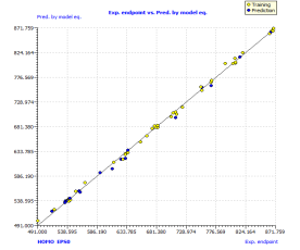
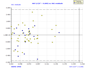
Figure 1. Scatter plot of experimental vs predicted boiling point (a), with the respective Williams plot (b).

The results (R²ysand Q²ys VS Kxy [35]) are plotted in Figure 2(b), where Kxy is the total correlation in the model variables (y included). The lower values of R²ys and Q²ys indicate the good results of the original model are not due to chance correlation or structural dependency of the training set. See (Table 2) the mean values of R²ys.

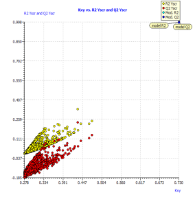
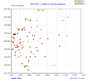
Figure2.Plot of Y-scrambling models compared with the originals model (a) and Insubria graph (plot of hat values vs. Predicted values for the whole set of PAHs) for the full QSPR model (b)

In order to exploit all the available information, we build up a full model from the complete data set. We used the same selected descriptor, which was demonstrated in the three splitting to be useful for the prediction of chemicals which were not used in model development. The full model, rigorously validated for its predictivity, can be applied to chemicals without experimental data in order to screen and prioritize them for future experiments or for filling the data gaps. For this reason, we applied our full model on 57 other PAHs without experimental availability for the boiling point. The Insubria graph (Figure 2b) shows that all these compounds are included in the model domain, considering the leverage approach. This demonstrates that this model has a great applicability to new PAHs, for which the predicted data are interpolated and therefore very reliable.

The comparison between the most important published models for boiling point prediction of PAHs [5-6,14-15], can be achieved using the table 3, It is easy possible to verify if one model is better than other, taking into account the size of the studied data set, the statistical parameters taken into considerations and the complexity of model (i.e. number of descriptors involved and the statistical modeling method), the model developed in this work includes more compounds and fewer descriptors, in addition, our model(eq.7) was evaluated by using different statistical parameters compared with other models in the literature [5-6,14-15], the present MLR model shows better statistical quality and performance than previous works.

Table3. Comparison between previous works and this work for the boiling point.

Works	N	Size of model	Type of descriptors	R2(%)	R[a]	Q2LOO (%)	RMSEpr	SEP[b]	Q²F1(%) Q²F2(%) Q²F3(%)
C.M.White[14]	47	1	The first-order valence molecular connectivity 1Xv,	–	0.994	–	–	8.59	–
Todeschini R, et al[6]	53	4	WHIM descriptors	95.9	–	95.0	17.4	–	–
M. Márcia, and C. Ferreira[5]	23	3	EA, Xv, Log W	–	0.9994	–	–	6.68	–
		3	EA, Xe, Log W	–	0.9993	–	–	5.52	–
		4	EA, Xe,  Xv, Log W	–	0.9995	–	–	5.70	–
		4	 EA, Xe, SArea, Log W	–	0.9996	–	–	4.40	–
Ferreira et al[15]	36	3	Volume (V), molecular weight (MW) and Randic connectivity index(R)	PLS model: 99.5	–	99.42	7.756	–	–
				PCR Model: 99.5	–	99.38	8.474	–	–
This work	61	2	EPS0 HOMO	99.8	–	99.8	4.756	4.790	99.80 99.73 99.75

Another comparison between calculated values of Bp using our model and that calculated by EPIWIN model [36] was done, table (1) summarizes results, giving the mean absolute error (MAE) and the root mean square error (RMSE) of the two models. The comparison in both cases is in favor of our QSPR model, due MAE_{QSPR model} (3.541) << MAE_EPIWIN (29.173) and RMSE_{QSPR model} (4.756) << RMSE_EPIWIN (37.647). This allows us to say that our model is a specialized model for the calculation of PAHs boiling point.

Descriptor contribution analysis and interpretation

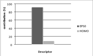
Figure.5 Relative contribution of selected descriptor to the MLR model

The relative model contributions of the two descriptors were determined and plotted in Figure 5. The significance of the descriptors involved in the model decreases in the following order: EPS0 (91.56 %) >HOMO (8.43 %). It should be noted that the difference in the descriptor contribution in the model is significant, we found that edge connectivity indices descriptor itself yielded a one-variable equation Bp= 252.5301+35.7598EPS0 with R² (%) = 99.71 and standard deviation s = 7.1002 K for n_tr = 42. This means that the edge connectivity indices descriptor used is an important descriptor for the influence of molecular structure on boiling point behavior for PAHs. However, a major drawback of edge connectivity indices is its degeneracy, i.e., isomers obtains identical numerical values. Hence, the model developed only by employing edge connectivity indices, is not accurate enough for PAHs. To improve the description a second regressor, HOMO, was added as shown above in [Eq. (7)].

The properties of PAH are a direct function of their size and topology. Size is a function of the number of π electrons, while topology is related to whether the ring systems are kata-annellated or peri-condensed. Topology is also a function of linear and angular ring annelation [19]. The PAH size and topology affect the energy of the highest occupied molecular orbital (HOMO), which in turn is a reasonable predictor of their properties.