Comparison of Gender Retailing in Australia

Business Statistics (ETC5900) Assignment

Question 1 – Retailing in Australia

1. The given data is cross sectional. This is because, the marketing company (Dynamic Marketing) has selected a random set of people (sample) from a large population and the data it provided to us is only a snapshot of the consumer behavior and only at one given point in time.

2. Purchase Preference – Categorical and Ordinal type of data

It is because a preference in general for any person means what the person likes more and in the case of the given data, purchase preference means, it is an option given to the sample to choose what they like more, i.e., Online shopping or In-store shopping. Therefore, even though purchase preference is just a label, it has an order associated to itself (Online shopping is preferred over In-store shopping or vice versa). It specifies an order in which the consumers would think of purchasing any product.

Gender – Categorical and Nominal type of data

A Nominal type of data classifies data into various distinct categories in which no ranking is implied. (Berenson, 2016)

Gender cannot have a ranking, i.e., we cannot say that women are better than men are or visa versa. Therefore, gender is only a label and cannot be ranked.

Mode of Purchase by Males and Females
Mode of Purchase	Gender		Grand Total
	Female	Male
In-store Online	39 54	55 52	94 106
TOTAL	93	107	200

(c)

4. The table above (part c) shows the frequency distribution of mode of purchase – In-store or Online shopping, by the two gender groups – Female and Male. The sample consists of 200 respondents out of which 93 are female respondents and 107 are male respondents.

Out of the 200 respondents, 94 prefer purchasing from an actual physical store. While, 106 prefer online shopping.

Out of the 93 females in the sample, 39 prefer shopping from physical stores and 54 prefer an online store.

In the case of male respondents, 55 men prefer shopping in-store and 52 prefer shopping online.

5. The mode of purchase most preferred by females is the online mode of purchase. Out of the 93 women in the sample, 54 (58%) make their purchases online and only 39 (42%) women choose to make their purchases from a store. Hence, online shopping is the most preferred mode of purchase.

For men, the most preferred mode of purchase is the in-store method. Out of the 107 men, 55 (51%) make their purchases from a store and only 52 (49%) make their purchases online. Even though the difference between the two methods is negligible, we must still consider that the preferred mode of purchase by the sample men is an in-store purchase.

(f)

Male – Income ($)
Mean	69,064.49
Median	67,500
Standard Deviation	17,510.28
First Quartile	56,750
Third Quartile	82,500
Interquartile Range	25,750
Range	77,60­­0
Minimum	35,500
Maximum	113,100
Coefficient of Variation	25.35%

Female – Income ($)
Mean	67,165.59
Median	64,800
Standard Deviation	18,093.22
First Quartile	55,700
Third Quartile	82,300
Interquartile Range	26,600
Range	77,600
Minimum	35,500
Maximum	113,100
Coefficient of Variation	26.94%

 

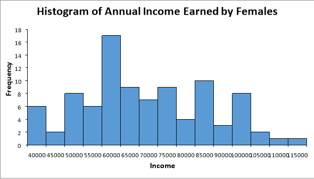
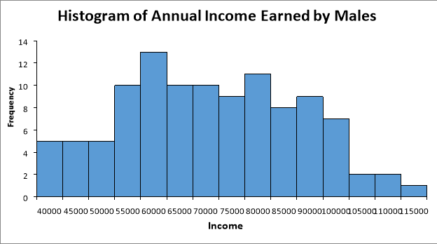
6. Central Tendency

The mean income for men ($69,064.49) is greater than the mean income earned by women ($67,165.59). The median income for men ($67,500) is also higher than that of women ($64,800). The modal class income for men and women ($60,000-$50,000) are the same. In conclusion, we can say that men earn more than women do. However, the difference is not very excessive. (Kaur, 2017a)

Variability

The range of income for men and women ($77,60­­0) is the same. This is because of the equal maximum ($113,100) and minimum ($35,500) salaries. The standard deviation of income for males ($17,510.28) is much smaller than females ($18,093.22). The range of the middle 50% of incomes for females ($26,600) is higher than for males ($25,750). The coefficient of variation reveals that the income for women (26.94%) has higher variability compared to the income of men (25.35%). Therefore, we can conclude that the income of females is slightly more variable than that of males. (Kaur, 2017a)

Shape

The distribution of income for males and females is right-skewed. This is because the mean is greater than the median in both the cases. This means that in the case of both, men and women, a majority of them earn a lower income. Both the histograms of income are unimodal.(Kaur, 2017a)

(j)

Sum of Annual Expenditure on Electronic Items ($)
Mode of Purchase	Gender		Grand Total
	Female	Male
In-store Online	7,687 8,621	11,770 9,170	19,457 17,791
TOTAL	16,308	20,940	37,248

The table above shows the total expenditure on electronic items by males and females categorized by their mode of purchase. The total amount spent by males and females on electronic items is $37,248. The total amount spent by males is greater ($20,940) than females ($16,308) irrespective of their preferred mode of purchase. (Kaur, 2017b)

This is also accurate for the mode purchase. Male customers spend more when purchasing from a store ($11,770) compared to the female customers who purchase in-store ($7,687). The amount spent on in-store purchases is greater ($19,457) compared to online mode of purchase ($17,791). (Kaur, 2017b)

Question 2 – CK & Partners

1. The data provided is a time series analysis because the law firm has been collecting the data from a long period, i.e., per year. It is a series of data, which is been collected at equally spaced intervals.

2. Starting Salaries – Numerical and Continuous type of data

This is because it is a measurement of a person’s wealth. We cannot always represent starting salaries in the form of integers and it varies from person to person. It is sometimes highly unlikely that two people will receive the same starting salary.

Year – Categorical and Ordinal type of data

A year is a label. However, year can be ranked and has order. Therefore, it is a categorical and ordinal type of data.

 Eg:- 2015 will come before 2016, 2016 will come before 2017 and so on.

3. Since the data is a Time Series form of data, the most appropriate form of graphical representation would be a line chart. A time series data can be portrayed effectively on a line chart, as it shows the progression of the trend across time with the help of a continuous line.

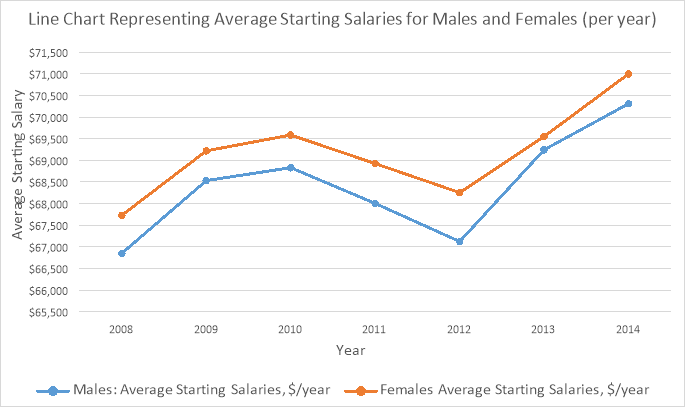
5. The general trend of average starting salaries for both, men and women have risen from 2008-2014. The trend began to decline after 2010 and reached its lowest in 2012 with an approximate decline of 2.50% for males and 2% for females. Since the decline, the average starting salaries have increased approximately 4.75% for men and 4% for women employees.

Throughout the years (2008-2014), women have had a higher average starting salary than men have – even during the decline in 2010. If the average starting salaries do not face another slump year, they are most likely to continue on their current path of growth.

6. It is true that male employees with an MBA degree as a total earn higher starting salaries over female employees with a similar degree. The chart in Fig 1 shows the average starting salaries of men and women (2008-2014) with an MBA degree and Fig 2 shows the level of employment for males and females (2008-2014).

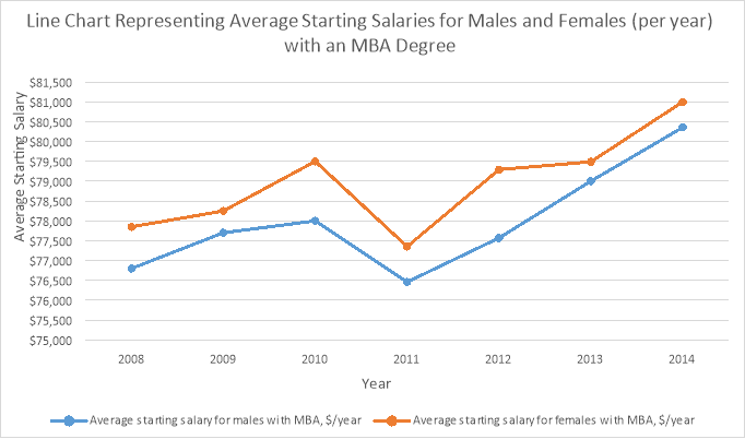
Fig 1

Even though it looks like women earn higher average starting salaries than men do, there is not much difference between the two. In-fact we are only provided with the average starting salaries for men and women in the IT company.

Average starting salaries is a very poor parameter to judge the actual gap in the starting salaries earned by the men and women of the company.

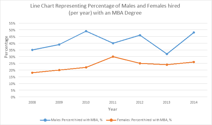
Fig 2

In Fig 2 we can clearly see that men with an MBA degree have a higher rate of employment at the company compared to women. Because of the large gap in employment, the difference in the average starting salaries of the men and women of the company becomes very insignificant.

Therefore, in conclusion, if we are to compare the actual starting salaries of males and females, we will discover that males in-fact do earn higher starting salaries than female employees. This will be proven correct even if we are to consider only the average starting salaries.

Question 3 – Net Household Income

1. If we compare the mean in both the data sets, we can find that the households are in-fact better off in 2010 compared to the year 2000. However, comparing the mean is not the appropriate way to measure the difference in this case, because the distribution is right skewed and the median is the best method of central tendency that can be used when comparing two skewed data sets.

Thus, by comparing the medians of the data sets, the households are worse off in 2010. Therefore, the statement put forward by the analysts is incorrect.

2.  I agree with the statement. The distribution in 2010 has a standard deviation of $45,799 compared to the standard deviation of $39,180 in 2000.

The variables are more spread out and distant from the mean in 2010 than 2000.

3. It is true that the poor households have become poorer in 2010. We can prove that by analyzing the values in the 1^st quartile. Just by comparing the values in the 1^st quartile, we can see a decline in the household income of the poor, from $17,850 to $13,250.

The rich households have also faced a decline in their household income from $70,850 to $67,750 (2000-2010). We can find this by comparing the values in the 3^rd quartile.

Therefore, the statement given the analysts is only partially correct. They have only compared the values in the 5^th and 95^th percentile, which is an inaccurate way to compare the two data sets. We cannot consider the 5^th and 95^th percentile as a measure of household income for the poor and rich households because they are far away from the 1^st quartile (25^th percentile) and 3^rd quartile (75^th percentile) respectively.

Bibliography

Berenson, M. L. a. (2016). Basic Business Statistics : Concepts and Applications (4th edition. ed.): Melbourne, VIC. : Pearson Australia.

Kaur, C. (2017a). ETC5900_S1_2017_T3_solutions, 4-5. Retrieved from

Kaur, C. (2017b). ETC5900_S1_2017_T3_solutions, 6-7. Retrieved from