Compressive Sensing: Performance Comparison of Measurement

Compressive Sensing: A Performance Comparison of Measurement Matrices

Abstract–Compressive sensing paradigm involves three main processes: sparse representation, measurement, and sparse recovery process. This theory deals with sparse signals using the fact that most of the real world signals are sparse. Thus, it uses a measurement matrix to sample only the components that best represent the sparse signal. The choice of the measurement matrix affects the success of the sparse recovery process. Hence, the design of an accurate measurement matrix is an important process in compressive sensing. Over the last decades, several measurement matrices have been proposed. Therefore, a detailed review of these measurement matrices and a comparison of their performances is needed. This paper gives an overview on compressive sensing and highlights the process of measurement. Then, proposes a three-level measurement matrix classification and compares the performance of eight measurement matrices after presenting the mathematical model of each matrix. Several experiments are performed to compare these measurement matrices using four evaluation metrics which are sparse recovery error, processing time, covariance, and phase transition diagram. Results show that Circulant, Toeplitz, and Partial Hadamard measurement matrices allow fast reconstruction of sparse signals with small recovery errors.

Index Terms– Compressive sensing, sparse representation, measurement matrix, random matrix, deterministic matrix, sparse recovery.

 As shown in Fig. 1. compressive sensing involves three main processes: sparse representation, measurement, and sparse recovery process. If signals are not sparse, sparse representation projects the signal on a suitable basis so the signal can be sparse. Examples of sparse representation techniques are Fast Fourier Transform (FFT), Discrete Wavelet Transform (DWT), and Discrete Cosine Transform (DCT) [11]. The measurement process consists of selecting a few measurements,  from the sparse signal that best represents the signal where. Mathematically, this process consists of multiplying the sparse signal by a measurement matrix. This matrix has to have a small mutual coherence or satisfy the Restricted Isometry Property. The sparse recovery process aims at recovering the sparse signal from the few measurements selected in the measurement process given the measurement matrix Φ. Thus, the sparse recovery problem is an undetermined system of linear equations, which has an infinite number of solutions. However, sparsity of the signal and the small mutual coherence of the measurement matrix ensure a unique solution to this problem, which can be formulated as a linear optimization problem. Several algorithms have been proposed to solve this sparse recovery problem. These algorithms can be classified into three main categories: Convex and Relaxation category [12-14], Greedy category [15-20], and Bayesian category [21-23]. Techniques under the Convex and Relaxation category solve the sparse recovery problem through optimization algorithms such as Gradient Descent and Basis Pursuit. These techniques are complex and have a high recovery time. As an alternative solution to reduce the processing time and speed up the recovery, Greedy techniques have been proposed which build the solution iteratively. Examples of these techniques include Orthogonal Matching Pursuit (OMP) and its derivatives. These Greedy techniques are faster but sometimes inefficient. Bayesian based techniques which use a prior knowledge of the sparse signal to recover the original sparse signal can be a good approach to solve sparse recovery problem. Examples of these techniques include Bayesian via Laplace Prior (BSC-LP), Bayesian via Relevance Vector Machine (BSC-RVM), and Bayesian via Belief Propagation (BSC-BP). In general, the existence and the uniqueness of the solution are guaranteed as soon as the measurement matrix used to sample the sparse signal satisfies some criteria. The two well-known criteria are the Mutual Coherence Property (MIP) and the Restricted Isometry Property (RIP) [24]. Therefore, the design of measurement matrices is an important process in compressive sensing. It involves two fundamental steps: 1) selection of a measurement matrix and 2) determination of the number of measurements necessary to sample the sparse signal without losing the information stored in it.

A number of measurement matrices have been proposed. These matrices can be classified into two main categories: random and deterministic. Random matrices are generated by identical or independent distributions such as Gaussian, Bernoulli, and random Fourier ensembles. These matrices are of two types: unstructured and structured.   Unstructured type matrices are generated randomly following a given distribution. Example of these matrices include Gaussian, Bernoulli, and Uniform. These matrices are easy to construct and satisfy the RIP with high probability [26]; however, because of the randomness, they present some drawbacks such as high computation and costly hardware implementation [27]. Structured type matrices are generated following a given structure. Examples of matrices of this type include the random partial Fourier and the random partial Hadamard. On the other hand, deterministic matrices are constructed deterministically to have a small mutual coherence or satisfy the RIP. Matrices of this category are of two types: semi-deterministic and full-deterministic. Semi-deterministic type matrices have a deterministic construction that involves the randomness in the process of construction. Example of semi-deterministic type matrices are Toeplitz and Circulant matrices [31]. Full-deterministic type matrices have a pure deterministic construction. Examples of this type measurement matrices include second-order Reed-Muller codes [28], Chirp sensing matrices [29], binary Bose-Chaudhuri-Hocquenghem (BCH) codes [30], and quasi-cyclic low-density parity-check code (QC-LDPC) matrix [32]. Several papers that provide a performance comparison of deterministic and random matrices have been published. For instance, Monajemi et al. [43] describe some semi-deterministic matrices such as Toeplitz and Circulant and show that their phase transition diagrams are similar as those of the random Gaussian matrices. In [11], the authors provide a survey on the applications of compressive sensing, highlight the drawbacks of unstructured random measurement matrices, and they present the advantages of some full-deterministic measurement matrices. In [27], the authors provide a survey on full-deterministic matrices (Chirp, second order Reed-Muller matrices, and Binary BCH matrices) and their comparison with unstructured random matrices (Gaussian, Bernoulli, Uniform matrices). All these papers provide comparisons between two types of matrices of the same category or from two types of two different categories. However, to the best of knowledge, no previous work compared the performances of measurement matrices from the two categories and all types: random unstructured, random structured, semi-deterministic, and full-deterministic. Thus, this paper addresses this gap of knowledge by providing an in depth overview of the measurement process and comparing the performances of eight measurement matrices, two from each type.

The rest of this paper is organized as follows. In Section 2, we give the mathematical model behind compressive sensing. In Section 3, we provide a three-level classification of measurement matrices. Section 4 gives the mathematical model of each of the eight measurement matrices. Section 5 describes the experiment setup, defines the evaluation metrics used for the performance comparison, and discusses the experimental results. In section 6, conclusions and perspectives are given.

Compressive sensing exploits the sparsity and compresses a k-sparse signal by multiplying it by a measurement matrix where. The resulting vector   is called the measurement vector. If the signal is not sparse, a simple projection of this signal on a suitable basis, can make it sparse i.e. where. The sparse recovery process aims at recovering the sparse signal given the measurement matrix and the vector of measurements. Thus, the sparse recovery problem, which is an undetermined system of linear equations, can be stated as:

(1)

Where is the, is a sparse signal in the basis , is the measurement matrix, and  is the set of measurements.

For the next of this paper, we consider that the signals are sparse i.e. and . The problem (1) then can be written as:

(2)

This problem is an NP-hard problem; it cannot be solved in practice. Instead, its convex relaxation is considered by replacing the by the . Thus, this sparse recovery problem can be stated as:

(3)

Where is the -norm, is the k-parse signal, the measurement matrix and is the set of measurements. 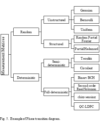Having the solution of problem (3) is guaranteed as soon as the measurement matrix has a small mutual coherence or satisfies RIP of order.

Definition 1: The coherence measures the maximum correlation between any two columns of the measurement matrix . If is a matrix with normalized column vector , each is of unit length. Then the mutual coherence Constant (MIC) is defined as:

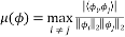(4)

Compressive sensing is concerned with matrices that have low coherence, which means that a few samples are required for a perfect recovery of the sparse signal.

Definition 2: A measurement matrix satisfies the Restricted Isometry Property if there exist a constant such as:

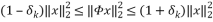(5)

Where is the and is called the Restricted Isometry Constant (RIC) of which should be much smaller than 1.

As shown in the Fig .2, measurement matrices can be classified into two main categories: random and deterministic. Matrices of the first category are generated at random, easy to construct, and satisfy the RIP with a high probability. Random matrices are of two types: unstructured and structured. Matrices of the unstructured random type are generated at random following a given distribution. For example, Gaussian, Bernoulli, and Uniform are unstructured random type matrices that are generated following Gaussian, Bernoulli, and Uniform distribution, respectively. Matrices of the second type, structured random, their entries are generated following a given function or specific structure. Then the randomness comes into play by selecting random rows from the generated matrix. Examples of structured random matrices are the Random Partial Fourier and the Random Partial Hadamard matrices. Matrices of the second category, deterministic, are highly desirable because they are constructed deterministically to satisfy the RIP or to have a small mutual coherence. Deterministic matrices are also of two types: semi-deterministic and full-deterministic. The generation of semi-deterministic type matrices are done in two steps: the first step consists of the generation of the entries of the first column randomly and the second step generates the entries of the rest of the columns of this matrix based on the first column by applying a simple transformation on it such as shifting the element of the first columns. Examples of these matrices include Circulant and Toeplitz matrices [24]. Full-deterministic matrices have a pure deterministic construction. Binary BCH, second-order Reed-Solomon, Chirp sensing, and quasi-cyclic low-density parity-check code (QC-LDPC) matrices are examples of full-deterministic type matrices.

Based on the classification provided in the previous section, eight measurement matrices were implemented: two from each category with two from each type. The following matrices were implemented: Gaussian and Bernoulli measurement matrices from the structured random type, random partial Fourier and Hadamard measurement matrices from the unstructured random type, Toeplitz and Circulant measurement matrices from the semi-deterministic type, and finally Chirp and Binary BCH measurement matrices from the full-deterministic type. In the following, the mathematical model of each of these eight measurement matrices is described.

A. Random Measurement Matrices

Random matrices are generated by identical or independent distributions such as normal, Bernoulli, and random Fourier ensembles. These random matrices are of two types: unstructured and structured measurement random matrices.

1) Unstructured random type matrices

Unstructured random type measurement matrices are generated randomly following a given distribution. The generated matrix is of size . Then M rows is randomly selected from N. Examples of this type of matrices include Gaussian, Bernoulli, and Uniform. In this work, we selected the Random Gaussian and Random Bernoulli matrix for the implementation. The mathematical model of each of these two measurement matrices is given below.

a) Random Gaussian matrix

The entries of a Gaussian matrix are independent and follow a normal distribution with expectation 0 and variance. The probability density function of a normal distribution is:

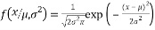(6)

Where is the mean or the expectation of the distribution, is the standard deviation, and is the variance.

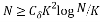
This random Gaussian matrix satisfies the RIP with probability at least given that the sparsity satisfy the following formula:

(7)

Where is the sparsity of the signal, is the number of measurements, and is the length of the sparse signal [36].

b) Random Bernoulli matrix

A random Bernoulli matrix is a matrix whose entries take the value or with equal probabilities. It, therefore, follows a Bernoulli distribution which has two possible outcomes labeled by n=0 and n=1.  The outcome n=1 occurs with the probability p=1/2 and n=0 occurs with the probability q=1-p=1/2. Thus, the probability density function is:

(8)

The Random Bernoulli matrix satisfies the RIP with the same probability as the Random Gaussian matrix [36].

2) Structured Random Type matrices

The Gaussian or other unstructured matrices have the disadvantage of being slow; thus, large-scale problems are not practicable with Gaussian or Bernoulli matrices. Even the implementation in term of hardware of an unstructured matrix is more difficult and requires significant space memory space. On the other hand, random structured matrices are generated following a given structure, which reduce the randomness, memory storage, and processing time. Two structured matrices are selected to be implemented in this work: Random Partial Fourier and Partial Hadamard matrix. The mathematical model of each of these two measurement matrices is described below:

a) Random Partial Fourier matrix

The Discrete Fourier matrix is a matrix whose entry is given by the equation:

(9)

Where.

Random Partial Fourier matrix which consists of choosing random M rows of the Discrete Fourier matrix satisfies the RIP with a probability of at least , if:

(10)

Where M is the number of measurements, K is the sparsity, and N is the length of the sparse signal [36].

b) Random Partial Hadamard matrix

The Hadamard measurement matrix is a matrix whose entries are 1 and -1. The columns of this matrix are orthogonal. Given a matrix H of order n, H is said to be a Hadamard matrix if the transpose of the matrix H is closely related to its inverse. This can be expressed by:

(11)

Where is the identity matrix, is the transpose of the matrix.

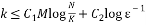
The Random Partial Hadamard matrix consists of taking random rows from the Hadamard matrix. This measurement matrix satisfies the RIP with probability at least provided  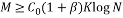 with and as positive constants, K is the sparsity of the signal, N is its length and M is the number of measurements [35].

B. Deterministic measurement matrices

Deterministic measurement matrices are matrices that are designed following a deterministic construction to satisfy the RIP or to have a low mutual coherence. Several deterministic measurement matrices have been proposed to solve the problems of the random matrices. These matrices are of two types as mentioned in the previous section: semi-deterministic and full-deterministic. In the following, we investigate and present matrices from both types in terms of coherence and RIP.

1) Semi-deterministic type matrices

To generate a semi-deterministic type measurement matrix, two steps are required. The first step is randomly generating the first columns and the second step is generating the full matrix by applying a simple transformation on the first column such as a rotation to generate each row of the matrix. Examples of matrices of this type are the Circulant and Toeplitz matrices. In the following, the mathematical models of these two measurement matrices are given.

a) Circulant matrix

For a given vector, its associated circulant matrix whose entry is given by:

(11)

Where.

Thus, Circulant matrix has the following form:

C=

If we choose a random subset of cardinality, then the partial circulant submatrix that consists of the rows indexed by achieves the RIP with high probability given that:

(12)

Where is the length of the sparse signal and its sparsity [34].

b) Toeplitz matrix

The Toeplitz matrix, which is associated to a vector   whose entry is given by:

(13)

Where. The Toeplitz matrix is a Circulant matrix with a constant diagonal i.e. .  Thus, the Toeplitz matrix has the following form:

T=

If we randomly select a subset of cardinality , the Restricted Isometry Constant of the Toeplitz matrix restricted to the rows indexed by the set S satisfies with a high probability provided

(14)

Where is the sparsity of the signal and is its length [34].

2) Full-deterministic type matrices

Full-deterministic type matrices are matrices that have pure deterministic constructions based on the mutual coherence or on the RIP property. In the following, two examples of deterministic construction of measurements matrices are given which are the Chirp and Binary Bose-Chaudhuri-Hocquenghem (BCH) codes matrices.

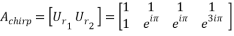
a) Chirp Sensing Matrices

The Chirp Sensing matrices are matrices their columns are given by the chirp signal. A discrete chirp signal of length 𝑚 has the form:

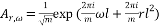
      (15)

The full chirp measurement matrix can be written as:

(16)

Where is an matrix with columns are given by the chirp signals with a fixed and base frequency  values that vary from 0 to m-1. To illustrate this process, let us assume that and

Given , The full chirp matrix is as follows:

 

In order to calculate, the matrices and should be calculated. Using the chirp signal, the entries of these matrices are calculated and given as:

;

 

Thus, we get the chirp measurement matrix as:

Given that is a -sparse signal with chirp code measurements and is the length of the chirp code. If

(17)

then is the unique solution to the sparse recovery algorithms. The complexity of the computation of the chirp measurement matrix is. The main limitation of this matrix is the restriction of the number of measurements to   [29].

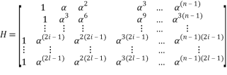
b) Binary BCH matrices

Let denote as a divisor of for some integer and as a primitive nth root of unity and assume that is the smallest integer for which divides If we set , then has order n. Define a code over by:

The BCH code is defined by:

(18)

BCH code can be also described in terms of a generator polynomial which is the smallest degree polynomial having zeros ,,. An example of binary matrices formed by BCH code is given as follows. Let n=15, p=4, and t=1, and let be a primitive element of satisfying:

(19)

 .

The BCH is the set of seven tuples that lies in the null space of the matrix

(20)

Since, a generating matrix is made from the coefficients 1101000 has the following form:

The binary BCH matrix presents some advantages such as simplicity of the sampling and reduction of the computational complexity. However, it does not meet the RIP requirement [41].

In this work, we have generated sparse signals of length N=1024. Then, we have sampled the sparse signals using the eight measurement matrices. The measurement signals were considered noisy. Gaussian noise with a standard deviation is added to the measurement signals.  Then sparse recovery of the original signal is performed using the Bayesian recovery via Fast Laplace technique. The choice of this sparse recovery algorithm is justified by the fact that it performs better than other sparse recovery algorithms, greedy and convex relaxation techniques [34]. In order to compare the performance of these measurement matrices, four evaluation metrics were used: recovery error, processing time, covariance, and phase transition diagram. Each of the experiments was repeated 100 times.

The recovery error calculates the error of reconstruction of the original signal. This metric is given by:

(21)

Where is the original sparse signal,  is the recovered signal, and is the.

Processing time of a measurement matrix is a metric that measures the time needed to perform the measurement given a sparse signal.

The covariance measures the correlation between the original signal and the recovered signal. It is given by:

(22)

Where E is the expectation,  is the original sparse signal, and is the recovered signal.

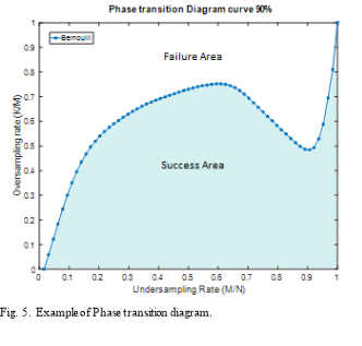
Another way to evaluate the performance of a measurement matrix is through its phase transition diagram. This diagram is a representation that separates the zone of failure and that of the sparse recovery process success. In order to generate a phase transition diagram, we generate a sparse signal with sparsity K. This signal is sampled using a measurement matrix. Then, recovery of the sparse signal is performed given the measurement matrix and vector of measurements. The same experiment is repeated 1000 times for the same value of the sparsity K and the number of measurement M, then the rate of success is calculated as:

(23)

Then, we vary the oversampling rate () and the undersampling rate from 0 to 1. Based on the success rate for different values of and δ, empirical phase-transition curve at 90% contour line is plotted. The same experiment is repeated for each of the eight measurement matrices. Finally, all these curves are plotted in the same graph in order to compare the performances of these measurement matrices. Fig. 2. presents an example of phase transition diagram. The x-axis corresponds to undersampling rate and the y-axis corresponds to oversampling rate (). The blue curve presents the curve that separates the area of success of the recovery process from its area of failure. The area bellow the curve present the zone of the success. For example if we consider and, we can say that based on the phase transition diagram of Bernoulli matrix, the recovery will be able to recover the signal. If we consider and, we can say that the recovery process will fail to reconstruct the original signal.

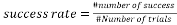
Examples of results are shown in Figs. 4 through 10. Fig. 4. shows the recovery Error of sparse recovery problem using Bayesian recovery algorithm via Fast Laplace with eight different measurement matrices with respect to the sparsity level of the signal. For a sparsity bellow 60, all measurement matrices have approximately the same performance and they all allow the recovery with a very small error except the Fourier measurement matrix that has a higher recovery error than all the other measurement matrices. For a sparsity greater than 60, the recovery error of the matrices, Binary BCH, Chirp, Circulant, Bernoulli, Gaussian, and Toeplitz, increases exponentially to become higher than that of the Random Pratiel Fourier measurement matrix when the sparsity order reaches the value 120. Binary BCH matrix and Random Pratiel Hadamard show better results than all measurement matrices for sparsity less than 100. For sparsity between 100 and 120, Toeplitz matrix performs better in term of recovery error and for a sparsity higher than 120 Random Pratiel Fourier matrix allows a recovery with the smallest error compared to all the other measurement matrices.

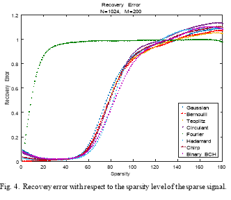
Fig .5 shows the recovery error with respect to the number of measurements. For a small number of measurements (M<=100), Random Partial Fourier matrix allow recovery with the smallest error among all the other measurement matrices. For a number of measurements higher than 85, the recovery errors of the Gaussian, Bernoulli, Toeplitz, Circulant, Hadamard chirp, and Binary BCH, decrease to become smaller than the one of the Random Partial Fourier matrix. All these measurement matrices, except the Partial Fourier matrix, have the same performance, but the Binary BCH and Partial Hadamard matrices show better performance than all the other matrices.

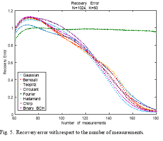
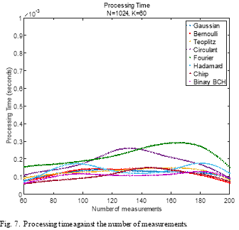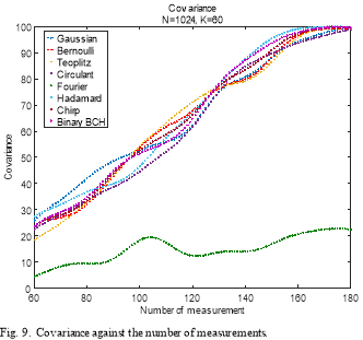
Fig. 6. shows the processing time of each of the eight measurement matrices considered in this comparison with respect to the sparsity level of the signal. As one can see, for a sparsity, the Partial Hadamard has the lowest processing time followed by Binary BCH, Gaussian, and Bernoulli. On the other hand, random Partial Fourier, Circulant,

and Toeplitz matrices require more time than all the other measurement matrices. As the sparsity increases the processing time decreases for all these matrices; however, random Partial Fourier, Circulant, and Toeplitz keep having the highest processing times and the random Partial Hadamard, Binary BCH, Gaussian, and Bernoulli have the lowest processing times.

Fig. 7. illustrates the processing time of the eight measurement matrices as a function of the number of measurements. As it can be seen from this figure, the Chirp measurement matrix has the smallest processing time, followed by circulant, Binary BCH, the Partial Hadamard, Bernoulli, Gaussian, and then Toeplitz. The Partial Fourier matrix requires more processing time than any other measurement matrices.

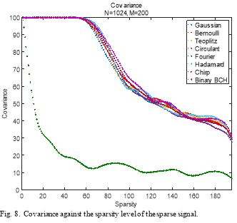
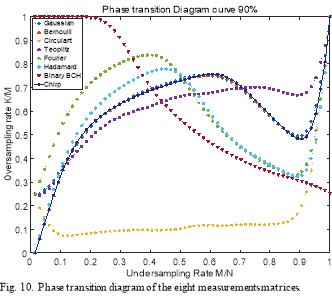Fig. 8. illustrates the covariance of the eight matrices as a function of the sparsity order of the sparse signal. All the measurement matrices have the same covariance shape except that of the random Partial Fourier.  For sparsity orders less than 60, the covariance is almost 100%, but it decreases exponentially for sparsity orders higher than 60. Among these measurement matrices, Binary BCH and Partial Hadamard matrices have the highest covariance values. On the other hand, Random Partial Fourier has the lowest value of covariance for all the sparsity values, which mean that this matrix performs less than all the other measurement matrices in term of covariance.

Fig. 9. shows the covariance of the eight measurement matrices with respect to the number of measurements. As can be observed, the covariance increases as the number of measurement increases to reach 100% except for the Partial Fourier matrix. It can also be observed that the covariance of all measurement matrices have slightly the same shape, except for the Random Partial Fourier matrix, which has the lowest value of the covariance for all value of measurements.

Fig. 10.  gives the phase transition diagram curves of the eight measurements matrices. These curves are obtained for a 90% of success rate of the recovery process. As can be seen, the curve of the Binary BCH matrix is above all the other curves for undersamling rate smaller than 0.4, which means that this measurement matrix has a higher success rate than the other measurement matrices. For higher undersampling rates, the curve of the Binary BCH matrix is below all the other curves, which means that this matrix has a lower success rate than the other measurement matrices. The curves of the Partial Fourier and Partial Hadamard are above the curves of random matrices for an undersampling rate smaller than 0.5. For a higher rate, these two curves are below the random matrices curves, Gaussian and Bernoulli curves. Toeplitz’s curve is above all the other curves for an undersampling rate higher than 0.7. The curve of the circulant matrix is below all the other curves, which means that it performs less than all the other measurement matrices.

Measurement matrices			Concept	Condition to satisfy the RIP	Strengths	weaknesses
Random	Structured	Gaussian	Entries follow a normal distribution		Simple and easy to implement Universal	Costly hardware implementation, More memory required
		Bernoulli	Entries are or with equal probability
	Unstructured	Partial Fourier	Randomly select rows from a discrete Fourier matrix		Easy to implement	Not accurate High uncertainty
		Partial Hadamard	Randomly select rows from Hadamard matrix		Fast recovery and Easy to implement	High uncertainty
Deterministic	Semi-deterministic	Circulant	Entries are distributed in one row and the rest of the matrix is generated by a simple rotation of the first row		Fast recovery ,Reduced randomness and memory usage	Not universal
		Toeplitz	Toeplitz matrix is a circulant with constant diagonal
	Full-deterministic	Chirp	Columns of this matrix are given by the chirp signals		Fast recovery	Restriction to a number of measurements:
		Binary BCH	Matrix formed by BCH code	Don’t satisfies the RIP yet	Simplicity of the sampling and Reduced computational complexity	Not accurate

Table. 1. gives a summary and comparison performance of the eight measurement matrices. As one can see, random measurement matrices are easy to implement and satisfy the RIP with high probability. However, they require more memory usage and present high computational complexity. Random

Partial Fourier matrix is not accurate and requires more number of measurements. Toeplitz and Circulant matrices are also simple to implement, allow fast recovery, and reduce the randomness. Deterministic matrices present the advantages of deterministic construction but they present some drawbacks. For example, chirp matrix is restricted to a number of measurement that should be the square of the length of the signal. The Binary BCH matrix do not satisfy the RIP.

In this paper, we have given an overview on compressive sensing paradigm, reviewed the measurement matrices, and classified them into two categories and four types. We described the implementation of each of the eight measurement matrices, two from each type. To compare the performances of

these matrices, we used four metrics, recovery error, processing time, covariance, and phase diagram. Experiment results show that deterministic measurement matrices have the same performance as the Gaussian and Bernoulli matrices. The Binary BCH and Random Partial Hadamard measurement matrices allow the reconstruction of sparse signals with small errors and reduce the processing time. Random Partial Fourier matrix with a high number of measurement performs better than all the measurement matrices considered in this work. Random measurement matrices perform well, but they present some drawbacks such as costly hardware and high memory storage. Deterministic measurement matrices perform better than random matrices; however, they have some weaknesses. For instance, the chirp matrix is restricted to a number of measurements that should be square the length of the signal and the Binary BCH matrix does not satisfy the RIP.

Acknowledgment

The authors acknowledge the support of the US Fulbright program.

