Debt Predictions Using Data Mining Techniques

Data Mining Project

Introduction

This report is set out to address the issue in which banks are facing. The project brief describes; the banks are finding it difficult to tackle debt and have leant out money to many people who promise to pay the loan back but never do. The banks says that they want to stop this happening. The banks have given some data of 2000 customers who have previously loaned money from them. Using this data, predictions will be made by using exploring different datamining techniques. This techniques will show predictions and differentiation between different types of loan customers, to outline how likely they will repay the loan. This will intern help predict in future how likely the customers will repay the loan. These are define on the attributes and results of each individual customer in the dataset given.

There are 2000 instances (customers) each within 15 attributes of this data set. Each customer is identified by a unique 6 digit customer ID.

Terminology Used

Standard division (StdDev) – a measure of quantity of how spread out numbers are and how much they differ from the mean.

A high standard deviation indicates that the data points are spread out over a wider range of values and are not close to the mean.

Outliers – Observations where noisy data occurs. It is not in correlation with the reset but could prove noteworthy.

Noise – modification of original values, an error or irrelevant data which should be removed.

Attribute – a property or characteristic of an object. Also known as a variable, field or characteristic.

Record – each row of the data set contains data variables.

Mean – the most common measure of the location of a set of points or the average of a set of numbers.

Instances – refers to the individual, custom or person that are identified by the unique ID. An instance has a set of values of 15 attributes.

Attributes

Customer ID, Forename, Surname, Age, Gender, Years at address, Employment status, Country, Current debt, Postcode, Income, Own home, CCJs, Loan amount, Outcome.

Data Summary

Attribute name	Datatype	Min	Max	Mean	Standard division	Values
Customer ID	Numeric	555574	1110985	837077.517	160763.319	Discrete
Forename	Nominal	Discrete
Surname	Nominal	Discrete
Age	Numeric	17	89	52.912	20.991	Continuous
Gender	Nominal	Discrete
Years at address	Numeric	1	560	18.526	23.202	Continuous
Employment status	Nominal	Discrete
Country	Nominal	Discrete
Current debt	Numeric		9980	3309.325	2980.629	Continuous
Postcode	Nominal	Discrete
Income	Numeric	3000	220000	38319	12786.506	Continuous
Own home	Nominal	Discrete
CCJs	Numeric		100	1.052	2.469	Continuous
Loan amount	Numeric	13	54455	18929.628	12853.189	Continuous
Outcome	Nominal	Discrete

Customer ID – used to uniquely identify their customer. After looking at the data it is evident that there are duplicating values. This data set indicates that the unique rate is 99%, therefor 14 values are duplicated or entered incorrectly. Deducting the Distinct value from the unique shows that 7 customers are duplicated in the system. Looking through the dataset, indicated that these customers have the same ID but different names, which is likely down to a mistake.

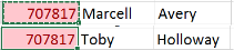Customers need to remain unique, if not this will affect other attributes which can contribute to the solution of repaying a loan problem as it will not reference the right customer data.

Forename Surname – these attributes cannot be used to give any sort of statistical material. They are not significant to giving any results of probability in terms of paying back loans in the future.

Filtering through the data set displays varying displays of data, which should not be allowed. This makes data filtering confusing and cluttered i.e. ‘E Spencer’. Some values also contain punctuation such as commas instead of apostrophe’s i.e. Dea,th. Also some of the genders for customers have been mixed up. Also an attribute for the gender has been mismatched i.e. Fewson has been assigned an F for female.

Age – there are no mistakes for customers within this attribute named age in this data set. The ages range from 1 7 ascending up to 89. 53 rounded up is the average age. The statistical information gives a good understanding of data provided. The StdDev of 20.991 shows a good spaced out data which is not clustered and unpredictable, surrounding the mean value.

The age group of 17 – 21; young age group in which a probable distribution can be used here. Or could use a different subset to give reliable data such as deviations in intervals of 10 years in difference.

This attribute Age can give statistical information on the accuracy of the age groups used with no external factors effecting their circumstances. If combining external factures attribute data such as ‘Debt Amount’ would give a very good and valuable probability statistics of these customers repaying loans in the future.

Gender – the dataset shows total of 9 variation of discrete values all of which represent male and female. Most of the data uses M and F for gender identification but H, D, and N are not known and be defined as ‘noise’. By looking at the forename, it is easy to identify the gender, therefore these error values can be changed accordingly.

‘Male’ and ‘Female’ attributed can be changed to ‘F’ and ‘M’ simply, as this is what they represent. Filtering through the datasheet shows that some forenames have been mismatched with the gender. These are assumed to have been entered in error and the genders have been altered correctly. There are four fields that have the value ‘Female’ but have male names i.e. Stuart, Dan, David, Simon these have therefore been changed to ‘M’. This may have occurred due to a misconfiguration issue.

After altering the data to the correct values the M and F gender percentage are very similar, with female = 48.45% and male = 51.55%, there is a 3.1% differentiation. This attribute can be used to give statistics accurately for predicting repayment of repayment of future loans. But although this could be true, discrimination based on gender will be obvious, therefore making the gender attribute inappropriate. This gender data will remain, though not all genders attributes can be accrue or 100% clear. The gender attribute can be said to be equal both ways and the usefulness of this is very low.

Again gender attributes usefulness is small. As stated above, the data can be entered inaccurately such as a forename which is presumed to be female is actually a male.

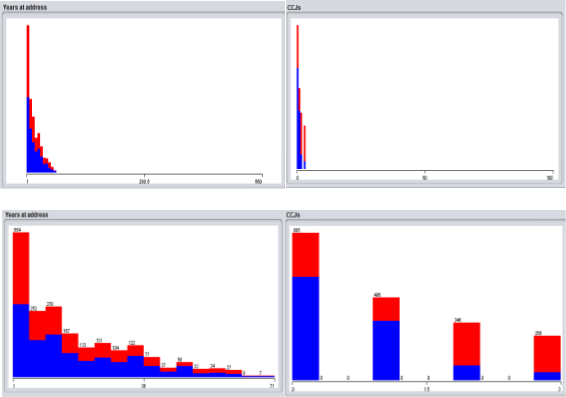
Years at address – There are 74 distinct values. Four anomalies appear to be in this attribute when scanning the dataset; Simon Wallace, Brian Humpreys, Steve Hughes, Chris Greenbank. These are showing an unlikely number of years living at an address for the customers. It is unclear as to whether the data was entered erroneously or if this number is indicative of months or days.

These values are shown as noise on the visualising screen for x: age y: years at address. As the dots lie outside the normal number of years range these are seen as not valid data.

If comparing the age and number of years at address, these four do not correlate therefore are deemed to be invalid data.

These customers should be removed from the data as they are unreliable sources of data. Removing these four would not affect anything as the figure is small and the remaining customers would provide reliable data.

It is believed that years at address would prove effective of the end result of probability of customer repaying a loan. And changing figures is not a good idea as it not clear what these figures are for.

If the data entered for these four is assumed to incorrect then, 71 would be the maximum years at address. To aid a solution to the problem, use a ten year interval subset for the Years at address attribute. It would give a reliable probability for the paying pack a loan, subject to the years living at the current address.

Employment status – the majority of the values in the employment status are dominated by self-employed. 1013 of 2000 people are self-employed which is 50.65%, 642 32.1% are unemployed, 340 17% are employed and 5 are retired 0.25%. It is not possible to prove the figures in the employment status attribute.

The retirement age is 65 but looking at the five people that are retired in this dataset, none of them are over this age. These customers that form the five retired customers are detached from the main body of customers and will be relevant in this dataset in determining the percentage of people which owe date and who have paid it back that are retired. This portion of the data set is very small therefore it is questionable of the reliability.

County – the county attribute contains 4 district values which are UK, Spain, Germany and France. The UK has most of the values (1994) and the rest of the six values are to the remaining countries.

There is not enough data to get an accurate or reliable result for Spain, Germany and France as the large portion of the data goes to the UK. With this, it would be possible to find a pattern in the UK customers but the usefulness is small in this therefore not suitable to building in the solution to the issue.

Current debt – 788 distinct values are contained within this attribute. There are 294 unique values (15%). A person cannot have a finite sum of debt, therefore it is continuous and the larger debt a person accumulates the harder it becomes for one to loan again or repay an outstanding loan.

In theory it is thought that a person with a large amount of debt and an income lower than their owed debt then they are less likely to make the repayment. This however is unproven.

Current debt attribute shows statistical facts of a person’s past debt and can be used to make a good prediction of the probability on whether a customer will pay back loans in future. When a person need to borrow money indicates they are struggling financially in which a loan was required to begin with can inferred the meaning of debt.

Post code – this attribute contains a total of 19171 attributes. It has no values missing (0%) therefore showing how there are more than one customer living in with one another or same area. These areas may form a pattern. As there aren’t enough subjects to form an accurate pattern and perception based on location cannot be allowed, likewise to gender.

This attribute cannot therefore hold any validity and cannot contribute to the solution of predicting loan repayment.

Income – this attribute contains 100 distinct and 0% at seven unique values. These values are continuous as income has no set amount and can salaries can vary i.e. with bonuses or overtime.

Income attribute is significant when evaluating alongside Current Debt. By predicting – a person on little income in whom has debt that they owe of the same figure, will not pay back future loans. By combining several attributes, trends can be seen i.e. those with less debt have a higher income. There are two outliers when viewing loan amount (y) and income (x) on the scatter graph. One has paid back loan and one has defaulted. As there are only two they may not affect the prediction in evaluating.

Own Home – contains three distinct values. There is no noise as there can be only three possible states for ownership of home and 0% missing values.

A prediction in people that are home owners in conjunction with having a high income will probable pay pack a loan. Therefore this attribute may contribute to providing data which can help predict repayment of future loans. From the evidence of the scatter graph in the income attribute a theory can be made; customers can repay a loan back whilst comfortable paying for a mortgage if they have a good wage and those that pay rent have out going expenses therefore find it difficult to repay loan.

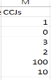CCJs – has six distinct values which range from 0 to 100. If a person has a customer has a CCJ then this indicates that the person is unreliable with repaying owed money back. The higher the number the higher risk the individual is in repaying a loan making this a vital factor within this dataset and would prove valuable in providing a probability result for repaying loans in future customers.

There are six distinct values 0, 1, 2, 3, 10 and 100. It can be assumed that 100 CCJs for this customer aged 27 is error data as this is highly unlikely, therefore would be regarded as noise. As the real value for this customer is unknown, this field can should be removed from the set and should assume it to be 1 or 10. As the other values 0, 1, 2 and 3 have numerous instances we could say the same for the person with 10 as there is a large gap between 3 and 10. 10 and 100 are unique out of 2000 customers.

Loan Amount – A loan amount can change continuously, no one person can have a set number of loans.

The lowest loan amount is 13 in the dataset. The lowest of the amount can be seen as input error values (noise) as the bank normally would not lend out such a low odd amount of £13. It is unsure what the real amount would be. It could be 1300

Outcome – contains distinct values of two; Paid and Defaulted attributes. This can be used to predict repayments of future loans of that customers.

Data Mining Algorithm Selection

Naïve Bayes

The first data mining algorithm selected is Naïve Bayes. It works on the Bayes theorem of probability named after Reverend Thomas Bayes in 1702-1761 to predict the class of an unknown dataset. It makes assumptions between features. The value of a particular feature is independent to the feature of another feature.

This classifier assumes that the presence of a particular feature in a class is unrelated to the presence of any other feature. [1]

Naïve Bayes has been used in real life scenarios where methods used for modelling in the area of diagnosing of diseases (Mycin). The method was applied to predict late onset Alzheimer’s disease in 1411 individuals whom each had 312318 SNP measurements available as genome-wide predictive features. This dealt with nonlinear dependant data and was proven to be powerful and affective in providing useful patterns in the large dataset [2].

The aim of this datamining technique is to determine whether a set of values of the attributes can be assigned to a particular class. It is worked out by finding the objects probability of its attributes values being a part of a particular class. The classifier is then determined as the most frequent possibility.

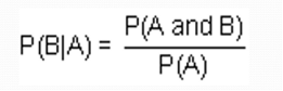
This annotation shows us the conditional probability. The probability that event B occurs so long as event A has already occurred is the conditional probability of event B in relation to event A.

The notation for conditional probability is P(B|A), read as the probability of B given A.

Zero frequency problem

One of the disadvantage with Naive-Bayes is that if you have no occurrences of a class label and a certain attribute value together then the frequency-based probability estimate will be zero. When all the probabilities are multiplied, it will give zero. Solution is to shift your zero frequency

Advantages & Disadvantages

Naive Bayes classifier makes a very strong assumption on the shape of your data distribution. The result of this can be bad. This is not all terrible as the Naive Bayes can be optimal even if the assumption is violated. If there are no occurrences of a class label and a certain attribute value together, then the frequency based probability estimate will be zero. Given Naive-Bayes’ conditional independence assumption, when all the probabilities are multiplied you will get zero and this will affect the posterior probability estimate.

Calculating probabilities is mostly overlooked, often trying to discretize the feature or fit a normal curve.

Naive Bayes gives useful outcomes with the algorithm being a robust method it can detect noise and unrelated attributes but Naive Bayes classification need big data set in order to make reliable estimations of the probability of each class. You can use Naïve Bayes classification algorithm with a small data set but precision and recall will keep very low.

to slightly higher. So, if you have counts of some occurrence in your data use Laplacian smoothing.

Decision tree

Decision trees are a representation for classification. It is a set of conditions, organized hierarchically in a way that the final decision can be determined following the conditions fulfilled from the root of the tree to one of its leaves. They are based on the strategy “divide and conquer”.

There are two phases for possible types of divisions. The first type is Nominal partition. Where an attribute may lead to a split with as many branches as vales there are for the attribute.

The second type is numeric partition. They allow partitions such as “x>” and “x <a” and partitions relating the two more than one attribute are disallowed.

A decision tree classifier is built in two phases.

The growth phase: The tree is constructed top down. It will find the “best” attribute. This is to be the root node and partitions are based on the attributes values. The method is applied to each partition. A node is highly pure if a particular class predominates amongst the examples at the node Decision tree methods are often referred to as Recursive Partitioning methods as they repeatedly partition the data into smaller and smaller – and purer and purer – subsets. Attributes representing nodes which are pure will be used and if this is not available the next most will be used. Pure nodes do not need to be split further as all sample of that node have the same class.

The pruning phase: the tree is pruned, bottom up. The processes of pruning the initial tree involves the removal of small and deep nodes resulted from noise within the training data which reduces the risk of “overfitting” which intern results in a more accurate classification of unknown data and makes the tree more general.

As the decision tree is being built the aim at each ode is to find out the split attributes and points that best divide the training records assigned to that leaf. The accuracy at which the classes are separated are defined by the value of a split.

ID3 was the first classification decision tree evolved by Ross Quinlan of 1986, which made some assumptions in the asic algorithm that all attributes are nominal and no unknown values. it was later improved to the C4.4 algorithm (an extension of ID3 algorithm) which was made to be more general in 1993.

Overfitting: The model performs poorly on new examples (e.g. testing examples) as it is too highly trained to the specific (non-general) nuances of the training examples.

Underfitting: The model performs poorly on new examples as it is too simplistic to distinguish between them (i.e. has not picked up the important patterns from the training examples)

Advantages and Disadvantages

Decision trees can be understood and conveyed easily, with diagrams being an advantage. A dataset can be too big, even to prune. This would make for a generation of a decision tree to become not generalised and very complicated.

Decision trees require minimal effort as they can be generated fast and can classify indefinite records.

A matter of pruning means that preparation of data is minimal. Pruning can deal with noise in the set and does not impact the majority of the accuracy of the generated tree. If the results are known then a white box model can be used, logic for the result can be used to understand the results. New scenario possibilities can be added.

C4.5

This algorithm is applied to problems in classification and makes a decision tree for the given training set. It is robust around noise and avoids overfitting. It deals with continuous, discrete attributes, missing data and converts trees into rules. It then minimizes the number of levels and tree nodes by pruning.

The c4.5 will work soundly with the dataset given by the bank as it contains attributes which are both continuous and discrete and also contains noisy data. This means that the noise values will not need removing as they would gain no impact on the final outcome.

The algorithm can be pruned to further enhance the findings. A training set of records whose class labels are known and used to build classification model. The classification model is applied to the test set that consists of records with unknown labels. The algorithm can further be tested to train the data with different methods for different viewpoints on the data set, such as cross validation, training sets and split 50:50

Impurity measures

Entropy measures impurity. In general the different impurity measures are consistent. The gain of a test condition: compare the impurity of the parent node with the impurity of the child nodes

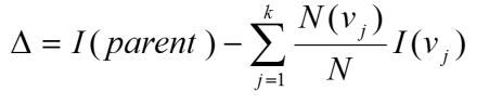
• Maximizing the gain == minimizing the weighted average impurity measure of children nodes
• If I() = Entropy(), then Δinfo is called information gain

Data Preparation

It has been outlined in the second chapter that some of the attributes; a person’s gender id and where a person lives have been discriminated and will not be included in this evaluation process of choosing if to give somebody a loan in future. The country attributes will not be used because the European countries do not have enough records to form an accurate pattern.

The attributes which will be used and are outlined in earlier chapter are; OutcomeIncomeLoan amountCCJsYears At AddressCurrent debtOwn homeAgeEmployment status.

And attributes not to be used; PostcodeSurnameForenameCustomer IDGenderCountry

Noise

There are six records which have effectively taken out of the data set giving a remaining amount as 1994 records.

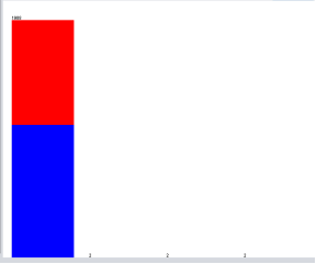
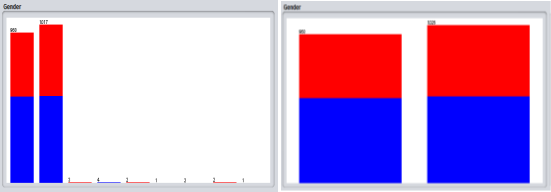The attribute ‘Gender’ has been updated to rectify the default values of the gender. The changes that were made was to change any full word ‘Male’ and ‘Female’ to F and M. the changes are represented in the histogram.

Pre edited histogram is to the left and post edited is beside it.

The six records were deleted are from the attributes named ‘Years at Address‘ and ‘CCJs’ cause these were seen as noise the evidence strongly suggests this by showing a person of the age of 27 having accumulated 100 CCJs in their life span it rather ridiculous assumption to base predictions on and a person aged 85 and having lived 560 years at his address is most certainly an error. By taking out these would not affect results as there are a vast quantity more data to make assumptions from.

CCJs and Years at Address histograms. These diagrams a displaying the before and after histogram charts, showing data as it has been updated. The top is the before and the bottom is post data removal.

Outliers

It can be predicted by inspecting the attribute named income that some curious material can be shown as these indicate some outliers. There are two contained within this attribute one is a value of 18000 and the other value at 220000 which are considerable different from the others. It can dawn to logical conclusion with this attribute as to whether one will fail succeed in making repayments of a loan in the future.

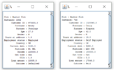
These two images depict at can assume that if the person is young (in their teens) has a vast income and they already have a CCJ then they are more likely to default however to a person that is middle aged with a large salary has never had a CCJ can assume they are more probable in repaying a loan.

As the outliers do not need removing from the Income attribute. The histogram shows the data set as it is:

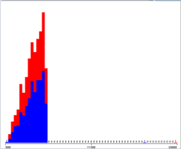
But after removing the records considered as noise from the CCJs and years at address attributes, it leaves the county attribute with six less records (1988) for UK residents. The six other values in the Countries attribute for France, Germany and Spain will be disregarded because the data is not enough to signify any real patterns.

Modelling Results and Discussion

Experiment 1: Investigate Training and Testing Strategies

Aim: – to investigate whether 50:50 or cross validation gives the best classification accuracy when using NB and J48

Methodologies

The parameter of the two chosen techniques for datamining will be altered in order to find the best most definite and purest outcome of data, this is when a particular technique will give the highest correctly classified instances. The C4.5 (J48 in Weka) and Naïve Bays algorithms will be tested.

50 50percentage split will be a testing option used for both techniques. To get reliable evaluation results, the test data must be different from the training data, therefore different independent samples. Percentage split, splits the data into a certain separate parts for learning and the rest of it for testing.

Using a split of 50 would prove best because all data is sampled equally without being bias however, using a larger portion split such as 80:20 would give a slight more accurate results for classification but the dataset from the bank is not large enough to base assumptions on its dependable statistics.

Cross validation (10 folds) will be another testing option which will be used against the two training algorithms. It fold the data into 10 folds and repeats it ten times (as there are the folds) the processes is as follows: 1 fold is used for testing and the remaining 9 folds are used for learning. Each time parting a different fold for testing and averaging out the results. Weka invokes the learning algorithm 11 times, one for each fold of cross validation and then a final time on the entire dataset.

Therefore out of 2000 records 1800 will be used for learning and 200 records used for testing

This method is the most reliable as it is a systematic way of improving upon repeated holdout by reducing the variants of the estimate.

Both of the methodologies J48 and Naïve Bayes will be testing using the testing methods descried above. More experiments will be conducted they will be compared to one another to see which combination provides the most correctly classified results.

Parameters

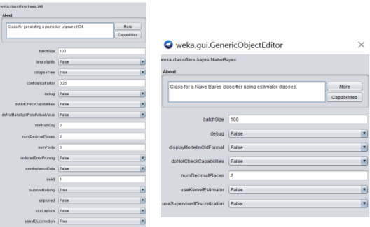For the initial testing, both Naïve Bayes and J48 parameters will remain at their default and unchanged as set in Weka, pictured below.

For the remaining experiments the parameters which will be changed are as follows:

J48 – binarySplits and unpruned.

Naïve Bayes – useKernalEstimtor and useSupervisdDiscretization.

It is important to change only one parameter at a time and log the confusion matrix and correctly classified instances and after, reverting the parameters back to their original state. Doing this ensures that the results are reliable and can distinguish which parameter made an effect.

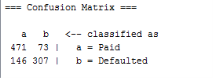
Confusion Matrix belowshows each of the data mining techniques used and for each strategy used. The table below shows the percentage for Paid and Default.

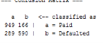
The table displays the results for percentages for the J48 and Naïve Bayes classifiers accuracy of correctly classified instances and the percentage for paid and default.

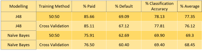
The table shows that the 50:50 training testing method gives the highest classification accuracy for both classifiers (J48 and Naïve Bayes), therefore these methods will be used correspondingly in the experimentations ahead.

Calculating the average for paid and default for each strategy combination in the table above shows, the model containing 50 50 J48 presents the average with the most at 77.35% which is the closes to its overall classification accuracy.

Experiment 2: Studying the Effects of Pruning

Aim: – to investigate whether pruning a decision tree gives the best classification accuracy when using J48.

Methodology

To see the effect on the correctly classified instances when setting the parameter unpruned to ‘true’.

Parameter

Originally the unpruned parameter is set at false therefore meaning that the tree was pruned. This time the parameter will be changed to false meaning that the tree will not be pruned. This will explore if changing the parameter has an effect on giving a more accurate classification.

The first investigation showed that a pruned tree produces a high percentage accuracy using split percentage at 50:50 in the J48 algorithm.

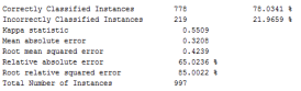
When changing the parameter to true, the accuracy reduces. The correctly classified instances becomes %77.03, dropping by %1.1.

Setting unpruned to true equates to a much larger decision tree.

Modelling	Training Method	% Paid	% Default	% Classification Accuracy
J48	50:50	85.84	66.44	77.03

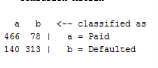
The paid attributes increases is percentage accuracy by 0.18% ad the paid attribute decreases its accuracy by 11.69%.

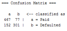
The confusion matrix above and the percentages in table show that the Deflated percentage is very low and the Paid is much higher.

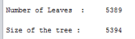
By setting the unpruned parameter to true, makes for a considerably larger decision tree.

If the bank used this large decision tree, they could utilise particular attributes more efficiently in providing valuable data should the bank wish to target customers for reasons of marketing: example, a customer whom is self-employed and is able to loan a higher figure as their current income has increased.

Experiment 3

Aim: – to investigate whether Binary Splits gives best classification accuracy when using J48.

Methodology

Binary Splits is set to ‘True’ this will evaluate whether a change in correctly classified percentage occurs.

Parameters used

Binary Splits is originally set to false. Setting it to true, Binary Splits, it creates two branches for multi-valued nominal attributes instead of one branch for each value upon constructing the tree.

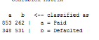
Using the J48 algorithm and 50:50 split percentage to form the decision tree. Binary splits gives a lower accuracy than when it isn’t in use. The results decline from %78.13 to 78.03, a reduction of %0.1.

The accuracy percentage for Paid is much greater than it is for default attribute as this remains still very low when using binarSplits. Although it is still higher than an unpruned tree but lower than the original settings of binarySplit set to false and unpruned set to false.

This time the tree is pruned resulting in a higher correctly classified instances. When it was unpruned, a lower percentage was presented therefore less reliable. By changing the unpruned parameter back to false and setting binarySplits to true, improved the percentage accuracy from experiment two although still not as accurate as the original parameters set in experiment one.

Also using the method of enabling the binarySplit equates to a more legible tree although it does present less tree branches of some attribute values.

Modelling	Training Method	% Paid	% Default	% Classification Accuracy
J48	50:50	86.58	67.77	78.03

The accuracy for the paid attribute has increased 0.92%.

Experiment 4: explore the effects of Kernel Estimator

Aim: – to investigate if the use of Kernel Estimator results in greater classification accuracy using Naïve Bayes.

Methodology

To change the Kernel Estimator parameter set to true in order to determine if this has a positive effecting in raising the correctly classified instances percentage. If the test raises the percentage then the parameter will remain set to true, else a negative less accurate percentage will result in the parameter being changed back to its default.

Parameters

‘False’ is the original parameter set for Kernel Estimator.

The Kernel estimator is the precision that numeric values are assigned.

The UseKernaelEstimator will be set to true, this means that the kernel estimator is used for numeric attributes instead of nominal.

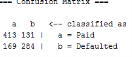
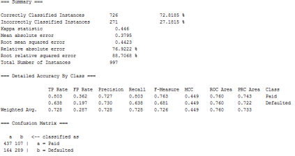
The set parameter are Naïve Bayes class and training option as Percentage split. The result increases when the Kernel Estimator is used. The classification accuracy is increased by 1.61% from 69.90% to 71.51%, therefore not using Kernel Estimator give a low classification accuracy than it does using it.

Un-normalised attributes in the dataset are dealt with by the Kernel Estimator allowing them to be levelled out.

Modelling	Training Method	% Paid	% Default	% Classification Accuracy
Naïve Bayes	50:50	79.59	61.81	71.51

To calculate the average, the sum of the paid and default are divided by 2 to give 70.7, which is very near to the classified accuracy of 71.51.

By applying the kernel estimator allowed for a higher accuracy percentage for just the paid attribute but not the default value. The paid value was increased by 3.68%, from 75.91% to 79.59% and the default attribute has dropped by 0.88% from 62.69 to 61.81% respectively.

This indicated that there was an advantage from applying this parameter but is not fully reliable as the paid percentage was lowered. It could therefore be used for further tests but with a combination of parameters changed to provide an optimum result.

Experiment 5: explore the efficacy of, Supervised Discretisation

Aim: – to find out stipulation of exhausting the use of supervised discretion to predict improvement for classification accuracy.

Methodology

The useSupervisedDiscretization parameter will be set to true to find out if correctly calssified instances percentage is confidently effected. Whether it is or not determines the whether it is kept or if the parameter it reverted back.

Parameters

This parameter is originally set at ‘false’, by changing it to ‘true’.

Discretization is a method for altering/separating continuous attributes, features or variables to discretized or nominal attributes, features, variables, intervals (Clarke, E. J.; Barton, B. A. (2000). “Entropy and MDL discretization of continuous variables for Bayesian belief networks”)

Supervised is a way of transforming numeric variable into categorised counterparts also referencing the class data when choosing discretization cut-points.

When Naïve Bayes classifiers, 50 50 percentages splits learning was used with the useSupervisedDiscretization set to true, the classification accuracy was higher than when it is not used. The correctly classified instances percentage accuracy has increased by 2.91% from 69.90% to 72.81%.

This test has shown that the effect of using supervised discretion has had a raise in the accuracy percentage, and had a positive bearing on both the values of ‘Paid’ and ‘Default’. So far, this is the first test which has had a fully progressive effect.

Modelling	Training Method	% Paid	% Default	% Classification Accuracy
Naïve Bayes	50:50	80.33	63.79	72.81

The percentage-accuracy for each attribute has been raised by 1 % from their first values of 75.91% to 79.59%.

Conclusion

It is evident to conclude that the J48 classifier using percentage split 50 50 gave the best outcome for correctly classified instances of both attributes for ‘Paid’ and ‘Default’. It had the highest percentage overall accuracy using the pre-set parameters.

Regardless of which parameter had been altered, the J48 gave the most desirable outcome in terms of the highest percentage accuracy more so than Naïve Bayes. Therefore J48 is the better classifier.

There are two experiments which caused a positive change in the accuracy percentage and these where experiments 4 and 5 using Naïve Bayes, Kernel Estimator and using supervised discretion (both observed separately). Enabling Kernel Estimator reduced only the accuracy of the default attribute by 0.88% and raised all other values. Switching Supervised Discretion to ‘true’ effected all the attributes and the accuracy percentage wholly.

Tests	Default	Pruning	Binary Splits	Kernel Estimator	Supervised Discretisation
J48 Percentage split Paid %	85.66	85.84	86.58	/	/
J48 Percentage split Defaulted %	69.09	66.44	67.77	/	/
Naive Bayes Percentage split Paid %	75.91	/	/	79.59	80.33
Naive Bayes Percentage split Defaulted %	62.69	/	/	61.81	63.79

Even though using Supervised Discretisation provided the only positive raise in attribute accuracy, it still lack by 5.33% for paid attribute In comparison to the Binary Splits classifier for paid and 11.24 percentage difference for defaulted attribute. Therefore the Binary Splits parameters classified more instances of these attributes correctly.

Whether the banks would be able to use specific attributes to target customers for marketing or targeting particular records of customers that appeal to them for a particular occasion, then the J48 classifier binary split and split percentage 5050 would be best suitable. This would allow for a legible and easy to de-sect tree that classifies attributes vigorously.

The attribute which the bank could focus on more would be defaulted in regards to the banks current concern. They would not dwell on the figure of the paid customs even if there is a contrasting difference on the accuracy of the paid such as: paid – 86.58% and defaulted – 67.77%. Though this is one way of assessing the banks accuracy percentage for just one attribute, this strategy would not be ideal in gaining dependable for both attributes. It would be far more efficient to gain balanced results for paid and defaulted such as: paid – 86.58% and defaulted – 82.77%. Nonetheless, which ever strategy is applied, the parameters set by default using J48 applying the 50:50 cross validation testing method yields the highest collective set of outcomes.

[2] http://scialert.net/fulltext/?doi=itj.2012.1166.1174&org=11