Exploring Optimal Levels of Data Filtering
It is customary to filter raw financial data by removing erroneous observations or outliers before conducting any analysis on it. In fact, it is often one of the first steps undertaken in empirical financial research to improve the quality of raw data to avoid incorrect conclusions. However, filtering of financial data can be quite complicated not just because of the reliability of the plethora of data sources, complexity of the quoted information and the many different statistical properties of the variables but most importantly because of the reason behind the existence of each identified outlier in the data. Some outliers may be driven by extreme events which have an economic reason like a merger, takeover bid, global financial crises etc. rather than a data error. Under filtering can lead to inclusion of erroneous observations (data error) caused by technical (e.g. computer system failure) or human error (e.g. unintentional human error like typing mistake or intentional human error like producing dummy quotes for testing).[1] Likewise, over filtering can also lead to wrong conclusions by deleting outliers motivated by extreme events which are important to the analysis. Thus, the question of the right amount of filtering of financial data, albeit subjective, is quite important to improve the conclusions from empirical research. In an attempt to somewhat answer this question, this seminar paper aims to explore the optimal level of data filtering.[2]
The analysis conducted in this paper was on the Xetra Intraday data provided by the University of Mannheim. This time-sorted data for the entire Xetra universe had been extracted from the Deutsche Börse Group. The data consisted of the historical CDAX components that had been collected from Data stream, Bloomberg and CDAX. Bloomberg’s corporate actions calendar had been used to track dates of IPO listing, delisting and ISIN changes of companies. Corporations not covered by Bloomberg had been tracked manually. Even though few basic filters had been applied (for e.g. dropping negative observations for spread/depth/volume), some of which were replicated from “Market Microstructure Database File”, the data remained largely raw. The variables in the data had been calculated for each day and the data aggregated to daily data points.[3]
The whole analysis was conducted using the statistical software STATA. The following variables were taken into consideration for the purpose of identifying outliers, as commonly done in empirical research:
- Depth = depth_trade_value
- Trading volume = trade_vol_sum
- Quoted bid-ask spread = quoted_trade_value
- Effective bid-ask spread = effective_trade_value
- Closing quote midpoint returns, which were calculated by applying Hussain (2011) approach:
rt = 100*(log (Pt) – log (Pt–1))
Hence, closing_quote_midpoint_rlg = 100*log(closing_quote_midpoint(n)) – log(closing_quote_midpoint(n-1)). Where closing_quote_midpoint = (closing_ask_price+ closing_bid_price)/2
Our sample consisted of the first fifteen hundred and ninety five observations, out of which two hundred observations were outliers. Only the first two hundred outliers were analyzed (on a stock basis chronologically) and classified as either data errors or extreme events. These outliers were associated with two companies: “313 Music JWP AG” and “3U Holding AG”. Alternatively, a different approach could have been used to select the sample to include more companies but the basics of how filters work should be independent of the sample selected for the filter to be free of any biases so for instance if a filter is robust, it should perform relatively well on any stock or sample. It should be noted that we did not include any bankrupt companies in our sample as those stocks are beyond the scope of this paper. Moreover, since we selected the sample chronologically on a stock basis, we were able to analyze the impact of these filters more thoroughly on even the non-outlier observations in the sample, which we believe is an important point to consider when deciding the optimal level of filtering. Our inevitably somewhat subjective definition of an outlier was:
Any observation lying outside the 1st and the 99th percentile of each variable on a stock basis
The idea behind this was to classify only the most extreme values for each variable of interest as an outlier. The reason why the outliers were identified on a per stock basis rather than the whole data was because the data consisted of many different stocks with greatly varying levels of each variable of interest for e.g. the 99% percentile of volume for one stock might be seventy thousand trades, while that of another might be three fifty thousand trades and so any observations with eighty thousand trades in both stocks might be too extreme for the first stock but completely normal for the second one. Hence, if we identified outliers (outside the 1st and the 99th percentile) for each variable of interest on the whole data, we would be ignoring the unique properties of each stock which might result in under or over filtering depending on the properties of the stock in question. An outlier could either be the result of a data error or an extreme event. A data error was defined using Dacorogna (2008) definition:
An outlier that does not conform to the actual condition of the market
The ninety four observations in the selected sample with missing values for any of the variables of interest were also classified as data errors.[4] Alternatively, we could have ignored the missing values completely by dropping them from the analysis but the reason why they were included in this paper was because if they exist in the data sample, the researcher has to deal with them by deciding whether to consider them as data errors, which are to be removed through filters or change them for e.g. to the preceding value and hence it might be of value to see how various filters interact with them. An extreme event was defined as:
An outlier backed by economic, social or legal reasons such as a merger, global financial crises, share buyback, major law suit etc.
The outliers were identified, classified and analyzed in this paper using the following procedure: Firstly, the intraday data was sorted on a stock-date basis. Observations without an instrument name were dropped. This was followed by creating variables for the 1st and 99th percentile value for each stock’s closing quote midpoint returns, depth, trading volume, quoted and effective bid-ask spread and subsequently dummy variables for outliers. Secondly, after taking the company name and month of the first two hundred outliers, while keeping in consideration a filtering window of about one week, it was checked on Google if these outliers were probably caused by extreme events or the result of data errors and classified accordingly using a dummy variable. Thirdly, different filters which are used in financial literature for cleaning data before analysis were applied one by one in the next section and a comparison was made on how well each filter performed i.e. how many probable data errors were filtered out as opposed to outliers probably caused by extreme events. These filters were chosen on the basis of how commonly they are used for cleaning financial data and some of the popular ones were selected.
4.1. Rule of Thumb
One of the most widely used methods of filtering is to use some “rule of thumb” to remove observations that are too extreme to possibly be accurate. Many studies use different rules of thumb, some more arbitrary than others.[5] Few of these rules were taken from famous papers on market microstructure and their impact on outliers was analyzed. For e.g.:
4.1.1. Quoted and Effective Spread Filter
In the paper “Market Liquidity and Trading Activity”, Chordia et al (2000) filter out data by looking at effective and quoted spread to remove observations that they believe are caused by “key-punching errors”. This method involved dropping observations with:
- Quoted Spread > €5
- Effective Spread/Quoted spread > 4.0
- % Effective Spread/%Quoted Spread > 4.0
- Quoted Spread/Transaction Price > 0.4
Using the above filters resulted in the identification and consequent dropping of 61.5% of observations classified as probable data errors, whereas none of the observations classified as probable extreme events were filtered out. Thus, these spread filter looks very promising as a reasonably large portion of probable data errors was removed while none of the probable extreme events were dropped. The reason why these filters produced good results was because it looked at the individual values of quoted and effective spread and removed the ones that did not make sense logically rather than just removing values from the tails of the distribution for each variable. It should be noted that these filters removed all the ninety four missing values, which means that only five data errors were detected in addition to the detection of all the missing values. If we were to drop all the missing value observations before applying this method, it would have helped filter out only 7.5%[6] of probable data errors while not dropping any probable extreme values. Thus, this method yields good results and should be included in the data cleaning process. Perhaps, using this filter in conjunction with a logical threshold filter for depth, trading volume and returns might yield optimal results.
4.1.2. Absolute Returns Filter
Researchers are also known to drop absolute returns if they are above a certain threshold/ return window in the process of data cleaning. This threshold is subjective depending on the distribution of returns, varying from one study to another for e.g. HS use 10% threshold, Chung et al. 25% and Bessembinder 50%.[7] In case of this paper, we decided to drop (absolute) closing quote midpoint returns > |20%|. Perhaps, a graphical representation of time series returns of 313music JWP & 3U Holding can be used to explain why this particular threshold was chosen.
Figure 1. Scatter plot of closing quote midpoint return and date
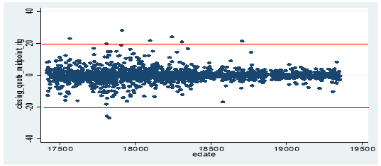
As seen in the graph, most of the observations for returns lie between -20% and 20%. However, applying this filter did not yield the best results as only 2.5% of probable data errors were filtered out as opposed to 10.3% probable extreme events from our sample. Therefore, this filter applied in isolation doesn’t really seem to hold much value. Perhaps, an improvement to this filter could be achieved by only dropping returns which are extreme but reversed[8] within the next few days as this is indicative of data error. For e.g. if T1 return= 5%, T2 return= 21% and T3 return=7%, we can tell that in T3 returns were reversed, indicating that T2 returns might have been the result of a data error. This filter was implemented by only dropping return values > |20%| which in the next day or two, reverted back to the value of return, +/- 3%[9]of the day before the outlier occurred as shown below:
r(_n)> |20%|
|r(n-1) -r(n+1)|<3%
|r(n-1) -r(n+2)|<3%
Where r(_n) is closing quote midpoint return on any given day. This additional filter seemed to work as it prevented the filtering out of any probable extreme events. However, the percentage of filtered data errors from our sample fell from 2.5% to 1.9%. In conclusion, it makes sense to use this second return filter which accounts for reversals in conjunction with other filters for e.g. spread filter. Perhaps, this method can be further improved by using a somewhat more objective range for determining price reversals or an improved algorithm for identifying return reversals.
4.1.3. Price Filter
We constructed a price filter inspired by the Brownlees & Gallo (2006) approach. The notion behind this filter is to gauge the validity of any transaction price based on its comparative distance to the neighboring prices. An outlier was identified using the following algorithm:
| pi - μ | > 3*σ
Where pi is the log of daily transaction price, the reason why logarithmic transformation was used is because the standard deviation method assumes a normal distribution.[10] μ is the stock sorted mean and σ is the stock sorted standard deviation of log daily prices. The reason why we chose the stock sorted mean and standard deviation was that the range of prices vary greatly in our data set from one stock to another, hence, it made sense to look at each stock’s individual price mean as an estimate of neighboring prices. This resulted in filtering 56.5% of probable data errors which were all missing values. Thus, this filter doesn’t seem to hold any real value when used in conjunction with a missing value filter. Perhaps, using a better algorithm for identifying the mean price of the closest neighbors might yield optimal results.
4.2. Winsorization and Trimming
A very popular filtering method used in financial literature is trimming or winsorization. According to Green & Martin (2015a), p. 8, if we want to winsorize the variables of interest at α%, we must “replace the nα largest values by the nα upper quantile of the data, and the nα smallest values by the nα lower quantile of the data”. Whereas, if we want to trim the variables of interest by α%, we should simply drop observations outside the range of α% to 1- α%. Thus, winsorization only reduces extreme observations rather than dropping them completely like trimming. For the purpose this paper, both methods will have similar impacts on dropping outliers outside certain α%, hence, we will only analyze winsorization in detail. However, winsorization introduces an “artificial structure”[11] to the dataset because instead of dropping outliers it changes them, therefore, if this research was to be taken a step further for e.g. to conduct robust regressions, choosing one method over the other would depend entirely on the kind of research being conducted.
The matter of how much to winsorize the variables, is completely arbitrary,10 however, it is a common practice in empirical finance to winsorize each tail of the distribution “at 1% or 0.5%”.5 We first winsorized the variables of interest at the 1% level, on a stock basis, which led to limiting 100% of probable extreme events and only 42.9% of probable data errors. Even though intuitively it would make sense for all the identified outliers to be limited because the method used for identifying outliers for each variable considered observations which were either greater than the 99th percentile or less than the 1st percentile, and winsorizing the data at the same level should mean that all the outliers would be limited. However, this inconsistency in expectation and outcome results from the existence of missing values – winsorization only limits the extreme values in the data, overlooking the missing observations which have been included in data errors. We then winsorized the variables of interest at a more stringent level i.e. 0.5%, on a stock basis, which led to 51.3% of the identified data errors and 18.6% of probable extreme events to be limited which doesn’t exactly seem ideal as in addition to data errors, quite a large portion of extreme events identified was also filtered out. Taking this analysis a step further, the variables of interest were also winsorized on the whole data (which is also commonly done) as opposed to on a per stock basis, at the 0.5% and 1% level. Winsorizing at the 1% level led to limiting 51% extreme events, 24.2% data errors and an additional one thirty four observations in the sample not identified as outliers. This points toward over filtering. Doing it at the 0.5% level led to limiting 28% extreme events, 12.4% data errors and an additional seven observations in the sample not identified as outliers. Thus, it seems that no matter which level (1% or 0.5%) we winsorize on or whether we do it on a per stock basis or on the whole data, a considerable percentage of probable extreme events is filtered out. Of course, our definition of an outlier should also be taken into consideration when analyzing this filter. Winsorizing on a per stock basis does not yield very meaningful results as it clashes with our outlier definition. However, doing it on the whole data should not clash with this definition as we identify outliers outside the 1st and the 99th percentile of each variable on the data as a whole. Regardless, this filter doesn’t yield optimal results as a substantial portion of probable extreme events get filtered out. This is because this technique doesn’t define boundaries for the variables logically like the rule of thumb method, rather it inherently assumes that all outliers outside a pre-defined percentile must be evened out and outliers caused by extreme events don’t necessarily lie within the defined boundary. It must also be noted that the winsorization filter does not limit missing values which are also classified as data errors in this paper. Thus, our analysis indicates that this filter might be weak if we are interested in retaining the maximum amount of probable extreme events. Perhaps, using it with an additional filter for limiting missing values might yield a better solution if the researcher is willing to drop probable extreme events for the sake of dropping probable data errors.
4.3. Standard Deviations & Logarithmic transformation
Many financial papers also use a filter based on x times the standard deviation:
xi > μ + x*σ
xi < μ – x* σ
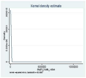
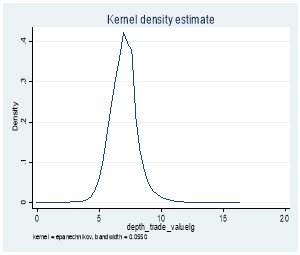
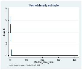
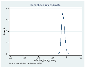
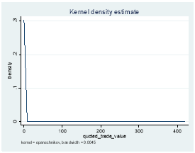
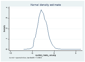
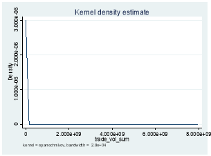
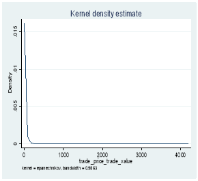
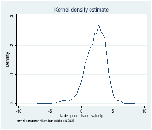
Where xi is any given observation of the variable of interest, μ is the variable mean and σ is variable standard deviation.[12] An example would be Goodhart and Figliuoli (1991) who use a filter based on four times the standard deviation.[13] However, this method assumes a normal distribution, 9 so problems might arise with distributions that are not normal and in our data set, except for returns (because we calculated them using log), the rest of the distributions for depth, trading volume, effective and quoted bid-ask spread are not normally distributed. Therefore, we first log transformed the latter four distributions using:
y = log (x)[14]
Where y is the log transformed function and x is the original function. The before and after graphs, using log transformation are shown in Exhibit 4. We then dropped observations for all the log transformed variables that were greater than Mean + x*Standard Deviation or less than Mean – x*Standard Deviation, first on a stock basis and then on the whole data for values of x=4 and x=6. Applying this filter at the x=6 level on a stock basis seemed to yield better results than applying it at the x=4 level. This is because x=6 led to dropping 25.6% less probable extreme events for a negligible 3.1% fall in dropping probable data errors. The outcomes are shown in Exhibit 3. However, upon further investigation, we found that 100% of the probable data errors identified by the standard deviation filter at the x=6 level were all missing values. This means that if we dropped all missing values before applying this filter at this level, our results would be very different as this filter would be dropping 7.7% extreme events for no drop in data errors.
Applying this filter on the whole data led to the removal of less outlier than applying it on a per stock basis. Using the x=6 level (whole data) appeared to yield the best results – 58.4% of probable data errors were filtered out while no probable extreme events were dropped. For more detailed results, refer to Exhibit 3. However, even in this case, 100% of the probable data errors identified were missing values. This means that if we were to drop all missing values before applying this filter, this filter would identify 0% of the probable extreme events or probable data errors. Thus, the question arises if we are actually over filtering at this level? If yes, then should x<6 be chosen? The answer to this question depends on how researchers treat missing values and like winsorization, whether they are willing to filter out some probable extreme events for the sake of getting rid of data errors.
Data cleaning is an extremely arbitrary process which makes it quite impossible to objectively decide the level of “optimal filtering”, which is perhaps, the reason behind limited research in this area. This limitation of research in this particular field and inevitably this paper should be noted. That being said, even though some filters chosen were more arbitrary than others, we have made an attempt to objectively analyze the impact of each filter applied. The issue of missing values for any of the variables should be taken into consideration because they are data errors and if we were to ignore them, they would distort our analysis because they interact with the various filters applied. Alternatively, we could have dropped them before starting our analysis, but we don’t know if researchers would choose to change them to the closest value for instance or filter them out, therefore, it’s interesting to see how the filters interact with them.
Our analysis indicates that when it comes to the optimal amount of data cleaning, rule of thumb filters fare better than statistical filters like trimming, winsorization and the standard deviation method. This is because statistical filters assume that any extreme value outside a specified window must be a data error and should be filtered out but as our analysis indicates, extreme events don’t necessarily lie within this specified window. On the other hand, rule of thumb filters set logical thresholds, rather than just removing/limiting observations from each tail of the distribution. The outcomes of different filters which are shown in exhibit 1, 2 and 3 are represented graphically below.
Figure 2. Box plot of outcomes of all the data cleaning methods
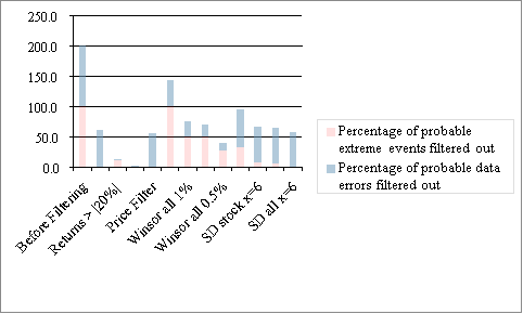
As shown in section 4.2 and the graph above, Winsorization whether on a stock basis or on the whole data, tends to filter out a large portion of probable extreme events. Thus, it is not a robust filter if we want to retain maximum probable extreme events and should be probably avoided if possible. As far as the standard deviation filter is concerned, as shown in section 4.3, applying it at the x = 6 level, whether on a per stock or whole data basis, seems to perform well but it is not of much value if combined with a missing values filter and all other scenarios tested, actually dropped more probable extreme events than data errors. Therefore, it is not advisable to simply drop outliers existing at the tails of distributions without understanding the cause behind their existence. This leaves us with the rule of thumb filters. We combined the filters that performed optimally – spread and additional return filter which accounts for reversals, along with a filter for removing the missing values. This resulted in dropping one hundred and two i.e. 63.4% of all probable data errors without removing any probable extreme events. At this point, a payoff has been made: in order to not drop any probable extreme events, we have foregone dropping some extra probable data errors because “over scrubbing is a serious form of risk”.[15] This highlights the struggle of optimal data cleaning, because researchers often don’t have the time to check the reason behind the occurrence of an outlier, they end up removing probable extreme events in the quest to drop probable data errors. Thus, the researcher has to first determine what “optimal” filtering really means to him – does it mean not dropping any probable extreme events albeit at the expense of keeping some data errors like done in this paper, or does it mean giving precedence to dropping maximum amount of data errors, albeit at the expense of dropping probable extreme events? In the latter case, statistical filters like trimming, winsorization and standard deviation method should also be carefully used.
The limitations of this paper should also be recognized. Firstly, only two hundred outliers were analyzed due to time constraint, maybe, future research in the area can look at a larger sample to get more insightful results. Secondly, other variables can also be looked at in addition to depth, volume, spread and returns and more popular filters can be applied and tested on them. Moreover, a different definition can be used to define an outlier or to select the sample for e.g. the two hundred outliers could have been selected randomly or based on their level of extremeness but close attention must be paid to avoid sample biases.
Future research in this field should perhaps, also focus on developing more objective filters and method of classifying outliers as probable extreme events. It should also look into the impact of using the above[16]two approaches of “optimal” filtering on the results of empirical research for e.g. on robust regressions, to verify which approach of “optimal” filtering performs the best.
Table 1: Outcome of Rule of Thumb Filters Applied
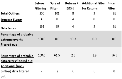
Table 2: Outcome of Winsorization Filters Applied
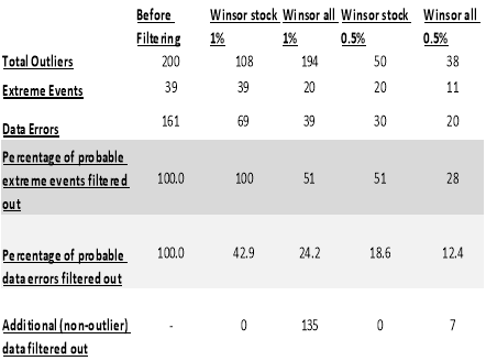
Table 3: Outcome of Standard Deviation Filters Applied
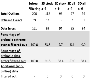
Figure 3: Kernel Distribution before and after log transformation
3.1 Depth
3.2 Effective Spread
3.3 Quoted Spread
3.4 Volume
 Â Â
  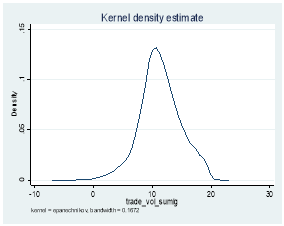
Figure 4. Kernel Distribution before and after log transformation of transaction price
 Â Â
References
Bollerslev, T./Hood, B./Huss, J./Pedersen, L. (2016): Risk Everywhere: Modeling and Managing Volatility, Duke University, Working Paper, p. 59.
Brownlees, C. T/Gallo, M. G. (2006): Financial Econometric Analysis at Ultra-High Frequency: Data Handling Concerns. SSRN Electronic Journal, p. 6
Chordia, T./Roll, R./Subrahmanyam, A (2000): Market Liquidity and Trading Activity, SSRN Electronic Journal 5, p. 5
Dacorogna, M./Müller U./Nagler R./Olsen R./Pictet, O (1993): A geographical model for the daily and weekly seasonal volatility in the foreign exchange market, Journal of International Money and Finance, p. 83-84
Dacorogna, M (2008): An introduction to high-frequency finance, Academic Press, San Diego, p. 85
Eckbo, B. E. (2008): Handbook of Empirical Corporate Finance SET, Google Books, p. 172
https://books.google.co.uk/books?isbn=0080559565
Falkenberry, T. N. (2002): High Frequency Data Filtering, S3 Amazon,
https://s3-us-west-2.amazonaws.com/tick-data-s3/pdf/Tick_Data_Filtering_White_Paper.pdf
Goodhart, C./Figliuoli, L. (1991): Every minute counts in financial markets, Journal of International Money and Finance 10.1
Green, C. G./Martin D. (2015): Diagnosing the Presence of Multivariate Outliers in Fundamental Factor Data using Calibrated Robust Mahalanobis Distances. University of Washington, Working paper, p. 2, 8
Hussain, S. M (2011): The Intraday Behaviour of Bid-Ask Spreads, Trading Volume and Return Volatility: Evidence from DAX30, International Journal of Economics and Finance, p. 2
Laurent, A. G. (1963): The Lognormal Distribution and the Translation Method: Description and Estimation Problems. Journal of the American Statistical Association, p. 1
Leys, C./Klein O./Bernard P./Licata L. (2013):Â Detecting outliers: Do not use standard deviation around the mean, use absolute deviation around the median, Journal of Experimental Social Psychology, p. 764
Scharnowski, S. (2016): Extreme Event or Data Error?, Presentation of Seminar Topics (Market Microstructure), Mannheim, Presentation
Seo, S. (2006): A Review and Comparison of Methods for Detecting Outliers in Univariate Data Sets, University of Pittsburg, Thesis, p. 6
Verousis, T./Gwilym O. (2010): An improved algorithm for cleaning Ultra High-Frequency data, Journal of Derivatives & Hedge Funds 15.4, p. 325
(2016): Xetra Intraday Database, Chair of Finance, University of Mannheim, p. 1
[1] Dacorogna (2008)
[2] Scharnowski (2016)
[3] “Xetra Intraday Database” (2013)
[4] In the later stage of the paper, we noticed that the standard deviation filter, price filter and spread filter were all identifying these missing values as outliers.
[5]Â Eckbo (2008), p. 173.
[6] Calculation: (5/(161-94))
[7] Verousis & Gwilym (2010)
[8] Bollerslev et al. (2016)
[9] We decided a +/- 3% window for reversion, inevitably arbitrarily.
[10]Â Leys et al. (2013)
[11]Â Green & Martin (2015b), p. 2.
[12] Dacorogna et al. (1993)
[13] Seo (2006)
[14] Laurent (1963)
[15] Falkenberry (2002)
[16] Refer to paragraph before the previous one.