Glaucoma Image Processing Technique
Team 19 Members
- 40102434 – Andrew Collins
- 40134357 – Connor Cox
- 40056301 – William Craig
- 40133157 – Aaron Devine
We have been tasked to develop a system that through image processing techniques would be able to detect glaucoma. This required us to enhance our knowledge in how to apply pre-processing, segmentation, feature extraction and post-processing on a set of given images to be able to produce a classification.
Glaucoma is an eye condition where the optic nerve, which is the connector from your brain to your eye becomes damaged. This can lead to a complete loss of vision if it is not detected and treated early on. This is caused by when fluid in the eye cannot be drained effectively which builds pressure and then applies excessive pressure on the optic nerve.
Detecting glaucoma normally is a very time consuming and expensive process because it requires a trained professional to carry out the research. The advantages of automating this process is that it frees up that professional’s time to carry out other duties.
The system is going to be tested methodologically during the creation of the assignment, to help us decide what would be the best parameters to use to help increase the detection rate of glaucoma.
System
The way we tackled this assignment is we made a system that takes image sets and converts them into data sets which trains and tests them through our classification process. The system assigns the data set to either being healthy or having glaucoma detected.  Training goes through the following stages in this order:
- Pre-processing.
- Segmentation
- Post-Processing.
- Feature Extraction
- Classification.
Methodology
For us to decide what would be the best choice of techniques for each stage of the system we are going to be using the a set methodology to standardize our selection process. The aim is to maximise the system to try and get it to yield the maximum correctness it can achieve at each stage so when it reaches the classification stage it would provide the most accurate result.
The best way we are going to measure the correctness of the system is running a testing/training cycle for each parameter being changed and put into a table and comparing them to select the best result.
Brightness Enhancement
In our system, I have implemented Automated Brightness Enhancement (ABE). ABE is used to normalise an image so the image’s mean gray value is equal to 127 or (255/2). The image below illustrates what the results look like.
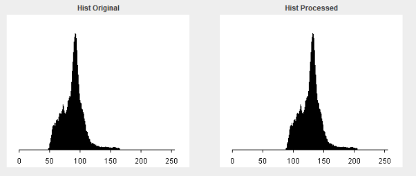

As you can see in the table above, the accuracy or our system significantly decreases when ABE is enabled. Therefore, for the good of the system’s accuracy, we will disable ABE in the system. As for why ABE damages the accuracy, it likely destroys some data within the images that have a more dynamic range than the one shown above. This would result in some gray levels being 0 or 255.
Accuracy significantly falls here. The reason for this is that ABE is causing the classifier to return positive for glaucoma for more images than it should, in turn, improving accuracy due to class ratio imbalance.
Contrast Enhancement
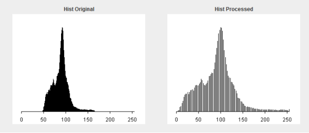
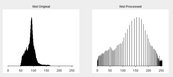
Our system implements three types of contrast enhancement, histogram equalisation, Automated Linear Stretch (ALS) and the Power Law. These three topics are covered extensively in the lecture slides, so in the interest of keeping the report concise, I won’t discuss them in depth here. Ultimately, only one of these techniques will be picked.
Automated Linear Stretch

Histogram Equalisation

Power Law
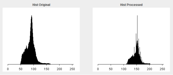
This example shows an error. The system doesn’t contain an automated way to find the value for  (gamma) in each image. So we’ll test every value of gamma from 0.0-2.0 in increments of 0.1 to see if any of our results provide a higher accuracy than when it isn’t enabled at all.
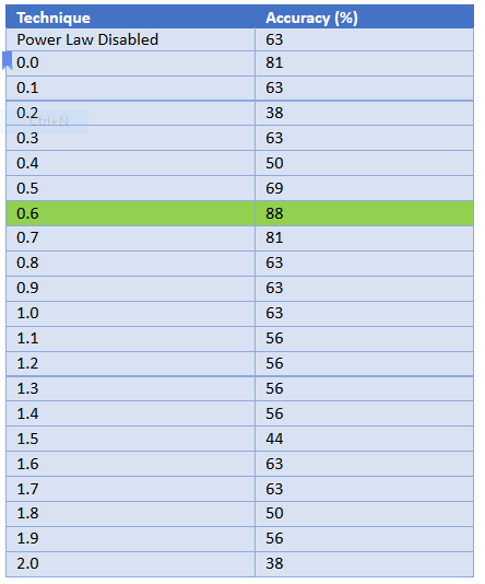
0.6, highlighted in green, shows that the accuracy is 88%,the image below shows power law being applied when there is an error.
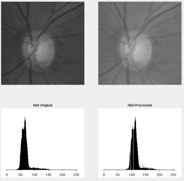
In the image above, the original image is the one on the left, and the processed image is on the right, and their corresponding histograms are underneath each, respectively. It would appear that the power law has actually made the dynamic range of our image worse.
Examining the segmented binary image below could explain why the accuracy has risen to 88%.
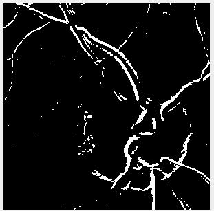
From this image, we can see that reducing contrast at the higher end, which seems to be what the error is doing, is allowing the segmenter, which is set at its default of edge extraction with a = 1 and no post processing, to detect the veins and optic nerve ring within the eye within the image with a higher level of success.
But why is this the case? it is due to the image’s background becoming more uniformed because of the reduction in contrast in the ‘white end’ while not altering the veins much at all as they are darker/greyer.
The reason values of y<0.6 produce poorer results is that the veins start being altered more effectively at 0.6, as the veins aren’t all that dark when the full available dynamic range is examined. From this, we could conclude that a system that darkens our image brightness without actually destroying/altering data in correspondence with the application of the power law with y<0.6 may achieve very high levels of accuracy.
Summary
From my tests, I have come to the conclusion that the best technique of the three is the Power Law. It was the only technique that improved our system’s accuracy. My tests also suggest that high levels of accuracy are dependent on the successful extraction of data about the veins, which, as I discussed above, the Power Law is highly effective at.
This theory makes even more sense when you consider that the other two methods, which significantly increased the dynamic range, did very poorly in comparison. Our system will benefit from using the Power Law, so from this point on it will be enabled.
Noise Reduction
Our system incorporates two kinds of noise reduction, those two being, Low Pass Filter and Median Filter. From examining our images, one would conclude that salt & pepper and CCD noise is not present. To demonstrate this however, we’ll need to see if the system gains accuracy when each technique is enabled.
Low Pass Filter (LPF)
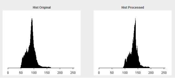

As we can see in the table above, accuracy has significantly decreased. To illustrate this, here is what the original and processed histograms look like when the contrast enhancement is applied without the low pass filter.

From the histograms, it would appear that low pass filter is actually removing some of the contrast enhancement. Low contrast seems to be mistaken for actual background noise, and when that happens, more distinct light and dark patches are created which in turn increases the dynamic range.
Median Filter
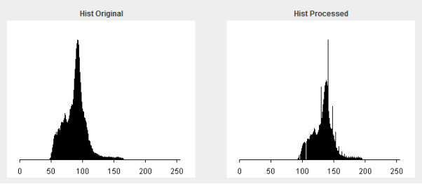

Similar to the low pass filter, the median filter is also removing some of the improvements made by contrast enhancement. Although it does appear that median pass filter is doing this to a lesser degree, as the accuracy is slightly higher here.
Summary
From our tests, we can conclude that both low pass filter and median pass filter only damage the accuracy of our system. LPF more so than MPF. It appears that the two actually undo some of the work done in contrast enhancement. As well as that, there isn’t actually enough noise in the image used here to warrant the use of a noise reduction filter at all.
After performing these tests, I decided to test my hypothesis, I tried applying the noise reduction filters before contrast enhancement to examine the results. The results were actually identical to the results from the earlier test. So what could that mean?
Well, it would seem that noise reduction is actually removing some information/data from the images, which then limits the effectiveness of the segmenter. From this point on, noise reduction filters will not be used.
Segmentation
This is used to separate the image into a foreground and a background with key areas in the foreground being turned white and the rest black. Our segmentation process involved using edge extraction and then automatic thresholding. The first thing we do is apply the Sobel mask to the pre-processed image
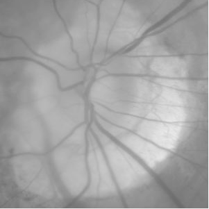
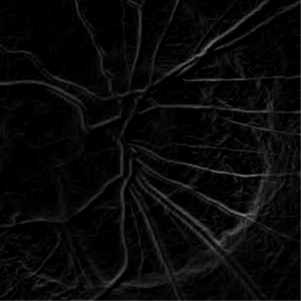
It’s very important to use edge extraction because it helps show the boundaries of the eye and make the veins much more defined. Right after that we apply automatic thresholding on the gradient magnitude image to get a binary segmented image.
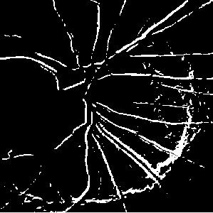
The class that we use to test which value to use is called SegmenterTest which will test the value of n within a range of -2.0 to 2.0 and increases the increments by 0.1 to see if the improved value increases the compared to a default value of n = 1. From this we got the following values:
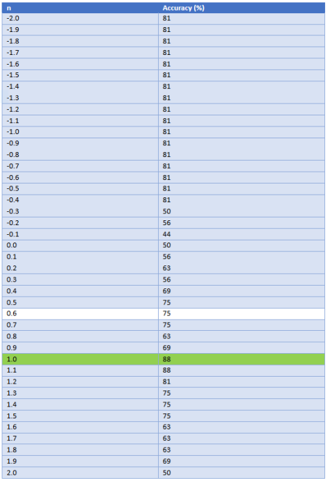
The default system where the value of n=1 it produces a good accuracy of 88% so this is the value that we pass into our segmenter.
This will allow more generic segmentation than what is possible with setting a manual threshold. The thresholds that are going to be in use are derived from the mean brightness of the pixels in the image raster and then adjusted by a standard deviation providing the best optional threshold for each image.
To check if Sobels Mask is the best for using to do edge extraction we will now compare the results from using Prewitt mask edge extraction.
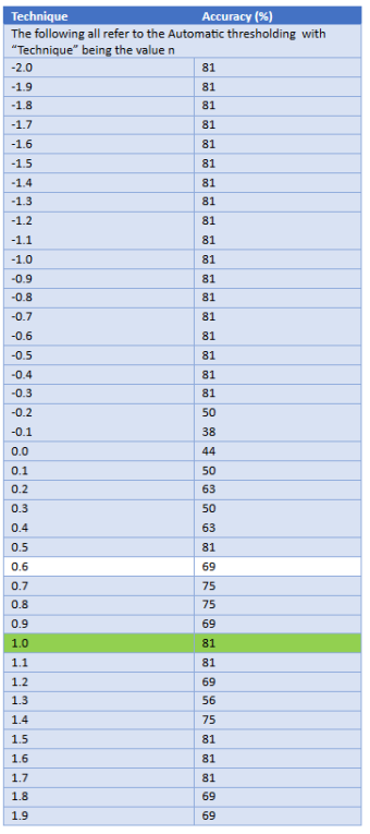
What we found that using the prewitt mask edge extraction as part of our segmentation process is that it is more effective using the default value on the Sobel Mask n = 1. The best accuracy that we got using the prewitt mask happens when we have n = 1 just like when we were using the sobel mask. This allows us to reduce that the sobel mask is the best option for us to use the edge extraction during the segmentation process.
Post-processing
Through this image processing technique, the image is enhanced and is filtered by a mask. The process uses erosion and dilation to remove isolated noise pixels, fills holes and smooth boundaries. Using brightness based segmentation, post processing is used to clean up the thresholded binary image. However, this can make objects appear smaller or larger than the original size.
We added the post processing techniques of closing and opening for our methods of erosion and dilation. To test which value that we are going to use we tried a variety of combinations and got the following results.
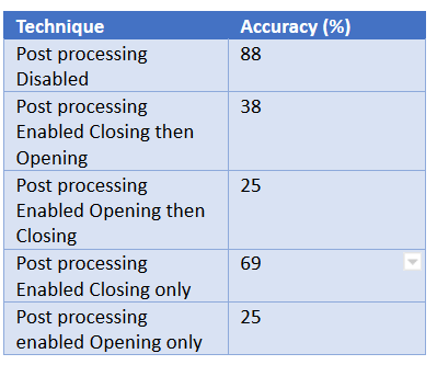
From what we gathered is that the best accuracy drops heavily when using any of the other post processing techniques were used.
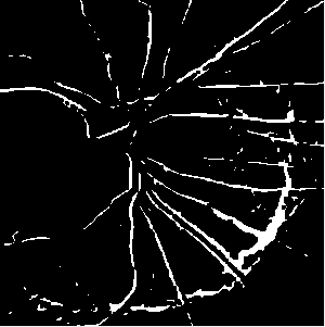
The image above has closing only enabled which produced the best accuracy from the post processing techniques however as you can tell by the image below which has post processing disabled it has much more detail. It is for this reason we will have post processing disabled because we are then able to receive better accuracy from the images. Post-processing did not have a positive result in the classification accuracy. It does make it visually easier to see how the application was processing the images.

Feature Extraction
The purpose of feature extraction is to gather useful features and details out of segmented images by extracting the feature vectors using a technique called moments. Implementing the use of moments correctly is the foundation for the essential calculations performed during the analysis of an object.
In our feature extraction class within our program we have decided that the following features of an object will be taken into consideration- Compactness, Perimeter, Position of Centroid and finally the Area of the object.
Before we perform the calculations for these features of said Object we first had to implement the moments formula in Java. Once we have created the moment method in our class we will then be able to use this to calculate the feature vectors needed.
Compactness
The reason we want to get the area and the perimeter is so that we can use the values to calculate what is needed, that being Compactness, as it is a more uself shape description for our vision system to use.. Compactness can be calculated by squaring the perimeter and then dividing it by the area.
private double compactness(BufferedImage image)
 {
      return Math.pow(getPerimeter(image), 2) / getArea(image);
 }
Above I have included the method that is called to calculate the compactness of the object, as you can see the calculation that was mentioned above is performed within this method.
Perimeter
We can get the object in question’s perimeter is first calculated by first eroding the object and then we perform a calculation to receive the new object’s area after erosion, after this we go onto calculating the difference between the new objects area and the initial objects area like so –
Perimeter = Original Area – Eroded Area
After this calculation is performed we are left with the perimeter of our object.
private double getPerimeter(BufferedImage image)
 {
return getArea(image) -Â Â Â Â Â Â Â Â Â Â Â getArea(PostProcessor.erode(image));
 }
I have placed the method used to get the perimeter of the object above, as you can see the method is performing the calculation required for the perimeter, Original Area – Eroded Area resulting in our perimeter.
Centroid Position
We can get the X & Y coordinates of the centroid in the object by performing the calculation of M01 & M10
private double [] position(BufferedImage image)
 {
      //calculate Centroid at M01
      double i = Math.round((moment(image, 0, 1))/ moment(image, 0, 0));
      //calculate Centroid at M10
      double j = Math.round((moment(image, 1, 0))/ moment(image, 0, 0));
      double [] Cij = {i, j};
      return Cij;
 }
Above is the method we have developed to find the position of the centroid for our Object. As you can see in the code above this method is using the moment method to perform the calculations needed to find the centroid position of the object.
 Area
We must also find the area vector, to do this we must calculate M00, this can be performed using the moment method which was developed earlier.
private double getArea(BufferedImage image)
 {
      return Math.round(moment(image, 0, 0));
 }
Above is a screenshot of the getArea method, this method calls upon the moment method and Math.round function to find the Area of our object.
Classification
Within our system which we have developed, we included the Nearest Neighbour function that is used to identify and recognise the training images we have supplied our system with. When we implement this feature in our system we get a variation of results depending on the value we set K to, we have included the results outputted by this function below for analysis –
Nearest Neighbour Function:
·        K = 1:
o   Accuracy: 62.50%
·        K = 3:
o   Accuracy: 87.50%
·        K =5:
o   Accuracy: 56.25%
As you can see in the above results from testing this function, the Nearest Neighbour Function provides us with the highest accuracy rate when using the value 3 for the K variable. This is due to the fact it can recognise the training images features. A disadvantage to this approach is that when changing the value of the K variable then this can alter the accuracy of the output as we can see when changing the value of K from 1 to 3, the accuracy increases greatly but once we change the value from 3 to 5 then the accuracy suffers and drops 30 points of accuracy.
Summary:
For this current group of images, the Nearest Neighbour function with the value K set to 3 is the best method used for classifying the object, this is because it returns the highest possible accuracy rate compared with other values of K such as 1 or 5, the accuracy rates for these values can be seen above.