HMMs Pattern Recognition

Assignment 3 of Pattern recognition is on HMMs. It should contain a detailed report on HMMs. The topics covered should include:

1. An introduction to HMM and its uses.

1. Problems of HMM, their explanation and relation to prior, posterior, and evidence.

2. Solution to the problems of HMM and their algorithms.

Pattern Recognition

Assignment # 3

Name: Muhammad Sohaib Jamal

An Introduction to HMM and it’s Uses

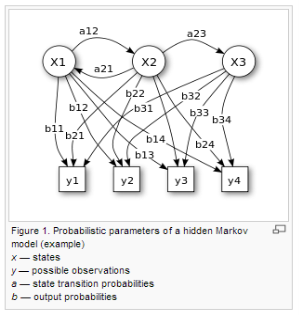
A Hidden Markov Model HMM is a stochastic model which has a series of observable variable X which is generated by hidden state Y. In an indirect way HMM consist of hidden states which has output that is comprised of a set of observations. Simple Markov Model models the states are directly observables means the states are directly output while in HMM the states are hidden and different form the observables or output. HMM is very reliable model for probabilistic estimation. HMM have applications in pattern recognitions such as speech recognition, gesture and hand writing recognition, computational Bioinformatics, etc.

Suppose we are considering three trails of a coin toss experiment and the person who is observing only know the results of the experiment when another person announces the result who is hidden in a closed room from the person noting the results. The result of this coin experiment can be any set of heads and tails e.g. THT, HHH, THH, TTT, THT etc. The person observing the results can get any sequence of heads and tails, and it is not possible to predict any specific sequence that will occur. The Observation Set is completely unpredictable and random.

1. Let’s assume that the third trail of coin toss experiment will produce more Head than the Tails. The resulting sequence will obviously have more number of heads then tails for this particular case. This is called “Emission probability” denoted by B_j(O).

2. Now we suppose that the chance of flipping the third trail after the first and second trail is approximately zero. Then, the transition from 1^st and 2^nd trail to 3^rd trail will be actually very small and as an outcome yields very little number heads if the person starts flipping the coin from 2^nd trail to 3^rd trail. This is called “Transition probability” denoted by a_ij.

3. Assume that each trail has some probability associated with the previous trail, then the person will start the process of flipping from that particular coin. This is known to be the “Initial probability” denoted by Ï€_i.

The sequence of number of heads or tails is known to be the observables and the number of trail is said to be the state of the HMM.

HMM is composed of:

• N number of hidden states S₁, S₂ ………., S_N

• M number of observations O₁, O₂, ……, O_M

• The Ï€_i (Initial state probability)

• Output Probability or Emission Probability B: P (O_M | S_N), where O_M is observation and S_N is the state.

• Transition probability matrix A = [ a_ij ].

• Transition probabilities a_ij.

• Mathematically the model is represented as HMM λ = {Π, A, B}

Problems of HMM and their explanations

HMM has three basic types of problems:

1. The Evaluation problem:

Suppose we have an HMM, complete with transition probabilities a_ij and output probabilities b_jk. We need to determine the probability that a particular sequence of observables states O_T was generated by that model.

2. The Decoding problem:

The transition probabilities, output probabilities and set of observations O_T is given and we want to determine the most likely sequence of hidden states S_T that led to those observations.

3. The Learning problem:

In such problem the number of states and observation are given but we need to find the probabilities a_ij and b_jk. With the given set of training observations, we will determine the probabilities a_ij and b_jk.

Relation of HMM to Prior, Posterior and evidence

The πi (Initial state probability) is analogous to the Prior probability. Because the initial probability is given before the set of experiments take place. This property of initial probability is identical to that of prior probability.

Similarly, the output probability or emission probability B: P (O_M | S_N) is analogous to the posterior probability. The posterior probability is used in forward backward algorithm.

In the same manner, evidence is the probability the next state is C given that the current state is state S_j. So the evidence is analogous to the transition probability A.

Solution to the problems of HMM and their algorithms

From the above mentioned discussion, we know that there are three different of problems in HMM. In this section we will briefly know how these problems are solved

1. Evaluation problem, this type of problem is solved the using Forward-Backward algorithm.

2. Decoding problem, for such type of HMM problem we use the Viterbi algorithm or posterior decoding

3. Training problem, in case of this type of problem we have the Baun-Welch re-estimation algorithm to solve it.

Forward-Backward algorithm

The forward and backward steps are combined by the Forward-Backward algorithm to estimate the probability of each state for a specific time t, and repeating these steps for each t can result in the sequence having the most likely probability. This algorithm doesn’t guarantee that the sequence is valid sequence because it considers every individual step.

The forward algorithm has the following three steps:

1. Initialization step
2. Iterations
3. Summation of overall states

.

Similarly, for backward algorithm we have the same steps like the forward algorithm:

1. Initialization step
2. Iterations
3. Summation of overall states

Viterbi algorithm

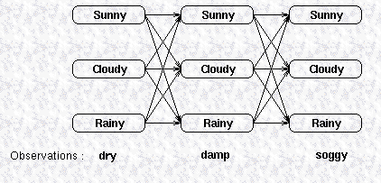
Viterbi algorithm is used to find the most likely hidden states, resulting in a sequence of observed events. The relationship between observations and states can be inferred from the given image.

In first step Viterbi algorithm initialize the variable

In second step the process is iterated for every step

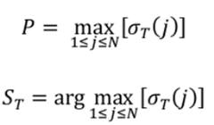
In third step the iteration ends

In Fourth step we track the best path

Baun-Welch re-estimation algorithm

Baun-Welch re-estimation algorithm is used to compute the unknown parameters in hidden Markov model HMM. Baun-Welch re-estimation algorithm can be best described using the following example.

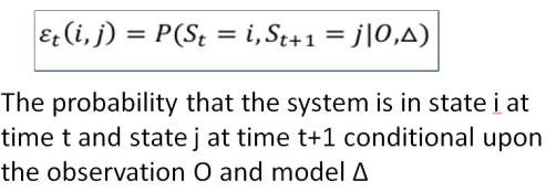
Assume we collect eggs from chicken every day. The chicken had lay eggs or not depends upon unknown factors. For simplicity assume that there are only 2 states (S1 and S2) that determine that the chicken had lay eggs. Initially we don’t know about the state, transition and probability that the chicken will lay egg given specific state. To find initial probabilities, suppose all the sequences starting with S1 and find the maximum probability and then repeat the same procedure for S2. Repeat these steps until the resulting probabilities converge. Mathematically it can be

References

1. Andrew Ng (2013), an online course for Machine learning, Stanford University, Stanford, https://class.coursera.org/ml-004/class.

2. Duda and Hart, Pattern Classification (2001-2002), Wiley, New York.

3. http://en.wikipedia.org

4. http://hcicv.blogspot.com/2012/07/hidden-markov-model-for-dummies.html

5. http://www.mathworks.com/help/stats/hidden-markov-models-hmm.html

6. http://www.comp.leeds.ac.uk/roger/HiddenMarkovModels/html_dev/viterbi_algorithm/s3_pg3.html