Lazy, Decision Tree classifier and Multilayer Perceptron

Performance Evaluation of Lazy, Decision Tree classifier and Multilayer Perceptron on Traffic Accident Analysis

Abstract. Traffic and road accident are a big issue in every country. Road accident influence on many things such as property damage, different injury level as well as a large amount of death. Data science has such capability to assist us to analyze different factors behind traffic and road accident such as weather, road, time etc. In this paper, we proposed different clustering and classification techniques to analyze data. We implemented different classification techniques such as Decision Tree, Lazy classifier, and Multilayer perceptron classifier to classify dataset based on casualty class as well as clustering techniques which are k-means and Hierarchical clustering techniques to cluster dataset. Firstly we analyzed dataset by using these classifiers and we achieved accuracy at some level and later, we applied clustering techniques and then applied classification techniques on that clustered data. Our accuracy level increased at some level by using clustering techniques on dataset compared to a dataset which was classified without clustering.

Keywords: Decision tree, Lazy classifier, Multilayer perceptron, K-means, Hierarchical clustering

1. INTRODUCTION

Traffic and road accident are one of the important problem across the world. Diminishing accident ratio is most effective way to improve traffic safety. There are many type of research has been done in many countries in traffic accident analysis by using different type of data mining techniques. Many researcher proposed their work in order to reduce the accident ratio by identifying risk factors which particularly impact in the accident [1-5]. There are also different techniques used to analyze traffic accident but it’s stated that data mining technique is more advance technique and shown better results as compared to statistical analysis. However, both methods provide appreciable outcome which is helpful to reduce accident ratio [6-13, 28, 29].

From the experimental point of view, mostly studies tried to find out the risk factors which affect the severity levels. Among most of studies explained that drinking alcoholic beverage and driving influenced more in accident [14]. It identified that drinking alcoholic beverage and driving seriously increase the accident ratio. There are various studies which have focused on restraint devices like helmet, seat belts influence the severity level of accident and if these devices would have been used to accident ratio had decreased at certain level [15]. In addition, few studies have focused on identifying the group of drivers who are mostly involved in accident. Elderly drivers whose age are more than 60 years, they are identified mostly in road accident [16]. Many studies provided different level of risk factors which influenced more in severity level of accident.

Lee C [17] stated that statistical approaches were good option to analyze the relation between in various risk factors and accident. Although, Chen and Jovanis [18] identified that there are some problem like large contingency table during analyzing big dimensional dataset by using statistical techniques. As well as statistical approach also have their own violation and assumption which can bring some error results [30-33]. Because of these limitation in statistical approach, Data techniques came into existence to analyze data of road accident. Data mining often called as knowledge or data discovery. This is set of techniques to achieve hidden information from large amount of data. It is shown that there are many implementation of data mining in transportation system like pavement analysis, roughness analysis of road and road accident analysis.

Data mining techniques has been the most widely used techniques in field like agriculture, medical, transportation, business, industries, engineering and many other scientific fields [21-23]. There are many diverse data mining methodologies such as classification, association rules and clustering has been extensivally used for analyzing dataset of road accident [19-20]. Geurts K [24] analyzed dataset by using association rule mining to know the different factors that happens at very high frequency road accident areas on Belgium road. Depaire [25] analyzed dataset of road accident in Belgium by using different clustering techniques and stated that clustered based data can extract better information as compared without clustered data. Kwon analyzed dataset by using Decision Tree and NB classifiers to factors which is affecting more in road accident. Kashani [27] analyzed dataset by using classification and regression algorithm to analyze accident ratio in Iran and achieved that there are factors such as wrong overtaking, not using seat belts, and badly speeding affected the severity level of accident.

2. METHODOLOGY

This research work focus on casualty class based classification of road accident. The paper describe the k-means and Hierarchical clustering techniques for cluster analysis. Moreover, Decision Tree, Lazy classifier and Multilayer perceptron used in this paper to classify the accident data.

1. Clustering Techniques

Hierarchical Clustering

Hierarchical clustering is also known as HCS (Hierarchical cluster analysis). It is unsupervised clustering techniques which attempt to make clusters hierarchy. It is divided into two categories which are Divisive and Agglomerative clustering.

Divisive Clustering: In this clustering technique, we allocate all of the inspection to one cluster and later, partition that single cluster into two similar clusters. Finally, we continue repeatedly on every cluster till there would be one cluster for every inspection.

Agglomerative method: It is bottom up approach. We allocate every inspection to their own cluster. Later, evaluate the distance between every clusters and then amalgamate the most two similar clusters. Repeat steps second and third until there could be one cluster left. The algorithm is given below

            X set A of objects {a1, a2,………an}

            Distance function is d1 and d2

            For j=1 to n

           dj={aj}

          end for

          D= {d1, d2,…..dn}

         Y=n+1

         while D.size>1 do

-(dmin1, dmin2)=minimum distance (dj, dk) for all dj, dk in all D

-Delete dmin1 and  dmin2  from D

-Add (dmin1, dmin2) to D

-Y=Y+1

          end while

K-modes clustering

Clustering is an data mining technique which use unsupervised learning, whose major aim is to categorize the data features into a distinct type of clusters in such a way that features inside a group are more alike than the features in different clusters. K-means technique is an extensively used clustering technique for large numerical data analysis. In this, the dataset is grouped into k-clusters. There are diverse clustering techniques available but the assortment of appropriate clustering algorithm rely on the nature and type of data. Our major objective of this work is to differentiate the accident places on their frequency occurrence. Let‘s assume thatX and Y is a matrix of m by n matrix of categorical data. The straightforward closeness coordinating measure amongst X and Y is the quantity of coordinating quality estimations of the two values. The more noteworthy the quantity of matches is more the comparability of two items. K-modes algorithm can be explained as:

                             d (X_i,Y_i)=                    —————–(1)

                Where           —————- (2)

2. Classification Techniques

Lazy Classifier

Lazy classifier save the training instances and do no genuine work until classification time. Lazy classifier is a learning strategy in which speculation past the preparation information is postponed until a question is made to the framework where the framework tries to sum up the training data before getting queries. The main advantage of utilizing a lazy classification strategy is that the objective scope will be exacted locally, for example, in the k-nearest neighbor. Since the target capacity is approximated locally for each question to the framework, lazy classifier frameworks can simultaneously take care of various issues and arrangement effectively with changes in the issue field. The burdens with lazy classifier incorporate the extensive space necessity to store the total preparing dataset. For the most part boisterous preparing information expands the case bolster pointlessly, in light of the fact that no idea is made amid the preparation stage and another detriment is that lazy classification strategies are generally slower to assess, however this is joined with a quicker preparing stage.

K Star

The K star can be characterized as a strategy for cluster examination which fundamentally goes for the partition of n perception into k-clusters, where every perception has a location with the group to the closest mean. We can depict K star as an occurrence based learner which utilizes entropy as a separation measure. The advantages are that it gives a predictable way to deal with treatment of genuine esteemed attributes, typical attributes and missing attributes. K star is a basic, instance based classifier, like K Nearest Neighbor (K-NN). New data instance, x, are doled out to the class that happens most every now and again among the k closest information focuses, yj, where j = 1, 2… k. Entropic separation is then used to recover the most comparable occasions from the informational index. By method for entropic remove as a metric has a number of advantages including treatment of genuine esteemed qualities and missing qualities. The K star function can be ascertained as:

K*(yi, x)=-ln P*(yi, x)

Where P* is the likelihood of all transformational means from instance x to y. It can be valuable to comprehend this as the likelihood that x will touch base at y by means of an arbitrary stroll in IC highlight space. It will performed streamlining over the percent mixing proportion parameter which is closely resembling K-NN ‘sphere of influence’, before appraisal with other Machine Learning strategies.

IBK (K – Nearest Neighbor)

It’s a k-closest neighbor classifier technique that utilize a similar separation metric. The quantity of closest neighbors may be illustrated unequivocally in the object editor or determined consequently utilizing blow one cross-approval center to a maximum point of confinement provided by the predetermined esteem. IBK is the knearest-neighbor classifier. A sort of divorce pursuit calculations might be used to quicken the errand of identifying the closest neighbors. A direct inquiry is the default yet promote decision blend ball trees, KD-trees, thus called “cover trees”. The dissolution work used is a parameter of the inquiry strategy. The rest of the thing is alike one the basis of IBL-which is called Euclidean separation; different alternatives blend Chebyshev, Manhattan, and Minkowski separations. Forecasts higher than one neighbor may be weighted by their distance from the test occurrence and two unique equations are implemented for altering over the distance into a weight. The quantity of preparing occasions kept by the classifier can be limited by setting the window estimate choice. As new preparing occasions are included, the most seasoned ones are segregated to keep up the quantity of preparing cases at this size.

Decision Tree

Random decision forests or random forest are a package learning techniques for regression, classification and other tasks, that perform by building a legion of decision trees at training time and resulting the class which would be the mode of the mean prediction (regression) or classes (classification) of the separate trees. Random decision forests good for decision trees’ routime of overfitting to their training set. In different calculations, the classification is executed recursively till each and every leaf is clean or pure, that is the order of the data ought to be as impeccable as would be prudent. The goal is dynamically speculation of a choice tree until it picks up the balance of adaptability and exactness. This technique utilized the ‘Entropy’ that is the computation of disorder data. Here Entropy is measured by:

                                 Entropy () = –

                                  Entropy () =

Hence so total gain = Entropy () – Entropy ()

Here the goal is to increase the total gain by dividing total entropy because of diverging arguments by value i.

Multilayer Perceptron

An MLP might be observed as a logistic regression classifier in which input data is firstly altered utilizing a non-linear transformation. This alteration deal the input dataset into space, and the place where this turn into linearly separable. This layer as an intermediate layer is known as a hidden layer. One hidden layer is enough to create MLPs.

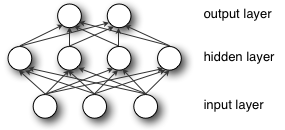
Formally, a single hidden layer Multilayer Perceptron (MLP) is a function of f: Y^I→Y^O, where I would be the input size vector x and O is the size of output vector f(x), such that, in matrix notation

                                                F(x) = g(θ⁽²⁾+W⁽²⁾(s(θ⁽¹⁾+W⁽¹⁾x)))

3. DESCRIPTION OF DATASET

The traffic accident data is obtained from online data source for Leeds UK [8]. This data set comprises 13062 accident which happened since last 5 years from 2011 to 2015. After carefully analyzed this data, there are 11 attributes discovered for this study. The dataset consist attributes which are Number of vehicles, time, road surface, weather conditions, lightening conditions, casualty class, sex of casualty, age, type of vehicle, day and month and these attributes have different features like casualty class has driver, pedestrian, passenger as well as same with other attributes with having different features which was given in data set. These data are shown briefly in table 2

4. ACCURACY MEASUREMENT

The accuracy is defined by different classifiers of provided dataset and that is achieved a percentage of dataset tuples which is classified precisely by help of different classifiers. The confusion matrix is also called as error matrix which is just layout table that enables to visualize the behavior of an algorithm. Here confusing matrix provides also an important role to achieve the efficiency of different classifiers.  There are two class labels given and each cell consist prediction by a classifier which comes into that cell.

Table 1

Confusion Matrix
                             Correct Labels
Negative	Positive
Negative	TN (True negative)	FN (False negative)
Positive	FP (False positive)	TP (True positive)

Now, there are many factors like Accuracy, sensitivity, specificity, error rate, precision, f-measures, recall and so on.

TPR (Accuracy or True Positive Rate) =

FPR (False Positive Rate) =

Precision =

Sensitivity =

And there are also other factors which can find out to classify the dataset correctly.

5. RESULTS AND DISCUSSION

Table 2 describe all the attributes available in the road accident dataset. There are 11 attributes mentioned and their code, values, total and other factors included. We divided total accident value on the basis of casualty class which is Driver, Passenger, and Pedestrian by the help of SQL.

Table 2

S.NO.	Attribute	Code	Value	Total	        Casualty Class
Driver	Passenger	Pedestrian
1.	No. of vehicles	1	1 vehicle	3334	763	817	753
2	2 vehicle	7991	5676	2215	99
3+	>3 vehicle	5214	1218	510	10
2.	Time	T1	[0-4]	630	269	250	110
T2	[4-8]	903	698	133	71
T3	[6-12]	2720	1701	644	374
T4	[12-16]	3342	1812	1027	502
T5	[16-20]	3976	2387	990	598
T6	[20-24]	1496	790	498	207
3.	Road Surface	OTR	Other	106	62	30	13
DR	Dry	9828	5687	2695	1445
WT	Wet	3063	1858	803	401
SNW	Snow	157	101	39	16
FLD	Flood	17	11	5
4.	Lightening Condition	DLGT	Day Light	9020	5422	2348	1249
NLGT	No Light	1446	858	389	198
SLGT	Street Light	2598	1377	805	415
5.	Weather Condition	CLR	Clear	11584	6770	3140	1666
FG	Fog	37	26	7	3
SNY	Snowy	63	41	15	6
RNY	Rainy	1276	751	350	174
6.	Casualty Class	DR	Driver
PSG	Passenger
PDT	Pedestrian
7.	Sex of Casualty	M	Male	7758	5223	1460	1074
F	Female	5305	2434	2082	788
8.	Age	Minor	<18 years	1976	454	855	667
Youth	18-30 years	4267	2646	1158	462
Adult	30-60 years	4254	3152	742	359
Senior	>60 years	2567	1405	787	374
9.	Type of Vehicle	BS	Bus	842	52	687	102
CR	Car	9208	4959	2692	1556
GDV	GoodsVehicle	449	245	86	117
BCL	Bicycle	1512	1476	11	24
PTV	PTWW	977	876	48	52
OTR	Other	79	49	18	11
10.	Day	WKD	Weekday	9884	5980	2499	1404
WND	Weekend	3179	1677	1043	458
11.	Month	Q1	Jan-March	3017	1731	803	482
Q2	April-June	3220	1887	907	425
Q3	July-September	3376	2021	948	406
Q4	Oct-December	3452	2018	884	549

1. Direct Classification Analysis

We utilized different approaches to classify this bunch of dataset on the basis of casualty class. We used classifier which are Decision Tree, Lazy classifier and Multilayer perceptron. We attained some result to few level as shown in table 3

Table 3

Classifiers	Accuracy
Lazy classifier(K-Star)	67.7324%
Lazy classifier (IBK)	68.5634%
Decision Tree	70.7566%
Multilayer perceptron	69.3031%

We achieved some results to this given level by using these three approaches and then later we utilized different clustering techniques which are Hierarchical clustering and K-modes.

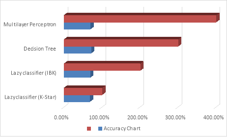
Figure 1  Direct classified Accuracy

2. Analysis by using clustering techniques

In this analysis, we utilized two clustering techniques which are Hierarchical and K-modes techniques, Later we divided dataset into 9 clusters. We achieved better results by using Hierarchical as compared to K-modes techniques.

Lazy Classifier Output

K Star: In this, our classified result increased from 67.7324 % to 82.352%. It’s sharp improvement in result after clustering.

Table 4

TP Rate	FP Rate	Precision	Recall	F-Measure	MCC	ROC Area	PRC Area	Class
0.956	0.320	0.809	0.956	0.876	0.679	0.928	0.947	Driver
0.529	0.029	0.873	0.529	0.659	0.600	0.917	0.824	Passenger
0.839	0.027	0.837	0.839	0.838	0.811	0.981	0.906	Pedestrian

IBK: In this, our classified result increased from 68.5634% to 84.4729%. It’s sharp improvement in result after clustering.

Table 5

TP Rate	FP Rate	Precision	Recall	F-Measure	MCC	ROC Area	PRC Area	Class
0.945	0.254	0.840	0.945	0.890	0.717	0.950	0.964	Driver
0.644	0.048	0.833	0.644	0.726	0.651	0.940	0.867	Passenger
0.816	0.018	0.884	0.816	0.849	0.826	0.990	0.946	Pedestrian

Decision Tree Output

In this study, we used Decision Tree classifier which improved the accuracy better than earlier which we achieved without clustering. We achieved accuracy 84.4575 % which is almost more than 15% earlier without clustering.

Table 6

TP Rate	FP Rate	Precision	Recall	F-Measure	MCC	ROC Area	PRC Area	Class
0.922	0.220	0.856	0.922	0.888	0.717	0.946	0.961	Driver
0.665	0.057	0.814	0.665	0.732	0.652	0.936	0.861	Passenger
0.868	0.027	0.841	0.868	0.855	0.830	0.988	0.939	Pedestrian

Multilayer Perceptron Output

In this study, our accuracy increased from 69.3031% to 78.8301% after using clustering technique.

Table 7

TP Rate	FP Rate	Precision	Recall	F-Measure	MCC	ROC Area	PRC Area	Class
0.929	0.338	0.796	0.929	0.857	0.627	0.892	0.916	Driver
0.452	0.036	0.824	0.452	0.584	0.520	0.855	0.720	Passenger
0.849	0.053	0.726	0.849	0.783	0.746	0.955	0.818	Pedestrian

We achieved error rate, precision, TPR (True positive rate), FPR (False positive rate), Precision, recall for every classification techniques as shown in given tables and also achieved different confusion matrix for different classification techniques. We can see the performance of different classifier techniques by the help of confusion matrix.

Here in the next table, we have shown the overall accuracy of analysis with clustering with the help of table 8, as we can compare this table from the previous table that our accuracy increased in each classification techniques after doing clustering.

Table 8

Classifiers	Accuracy
Lazy classifier (K-Star)	82.352%
Lazy classifier (IBK)	84.4729%
Decision Tree	84.4575%
Multilayer perceptron	78.8301%

We have shown accuracy level of table 8 in given figure 2 with the help of chart and we can see from the chart that it’s improved after doing clustering in accuracy chart also.

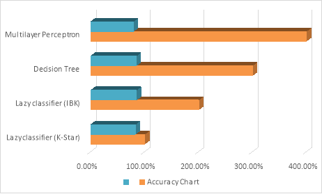
Figure 2 Accuracy after clustering

As we can see from table 3 and 8 that our accuracy level increased after clustering. We have shown comparison chart in fig. 3 without clustering and with clustering.

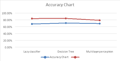
Figure 3 Compared accuracy chart with clustering and without clustering

6. CONCLUSION

In this study, we analyzed dataset without clustering and with clustering. We achieved better result when we used hierarchical clustering as compared to k mode clustering techniques.  We used different classifier such as Decision Tree, Lazy classifier and Multilayer perceptron to classify our dataset and they have shown optimized performance after clustering. We achieved better accuracy on the basis of casualty class (Driver, Passenger and Pedestrian) and we can see from tables that which factors are affecting more in accident on the basis of casualty class.

REFERENCES

1. Depaire B, Wets G, Vanhoof K. Traffic accident segmentation by means of latent class clustering. Accid Anal Prev.2008;40(4):1257-66.
2. Miaou SP. The Relationship between truck accidents and geometric design of road sections-poisson versus negative binomial regressions. Accid Anal Prev. 1994;26(4):471-82.
3. Miaou SP, Lum H. Modeling vehicle accidents and highway geometric design relationships. Accid Anal Prev. 1993;25(6):689-709.
4. Ma J, Kockelman K. Crash frequency and severity modeling using clustered data from Washington state. In: IEEE intelligent transportation systems conference. Toronto; 2006.
5. Savolainen P, Mannering F, Lord D, Quddus M. The statistical analysis of highway crash-injury severities: a review and assessment of methodological alternatives. Accid Anal Prev. 2011;43(5):1666-76
6. Abellan J, Lopez G, Ona J. Analyis of traffic accident severity using decision rules via decision trees. Expert Syst Appl. 2013;40(15):6047-54.
7. Kumar S, Toshniwal D. A data mining approach to characterize road accident locations. J Mod Transp. 2016;24(1):62-72.
8. Chang LY, Chen WC. Data mining of tree based models to analyze freeway accident frequency. J Saf Res. 2005;36(4):365-75.
9. Kashani T, Mohaymany AS, Rajbari A. A data mining approach to identify key factors of traffic injury severity. Promet- Traffic Transp. 2011;23(1):11-7.
10. Kumar S, Toshniwal D. Analyzing road accident data using association rule mining, International conference on computing, communication and security. Mauritius: ICCCS-2015; 2015. doi:10.1109/CCCS.2015.7374211
11. Oña JD, López G, Mujalli R, Calvo FJ. Analysis of traffic accidents on rural highways using latent class clustering and Bayesian networks. Accid Anal Prev. 2013;51(2013):1-10.
12. Kumar S, Toshniwal D. A data mining framework to analyze road accident data. J Big Data. 2015;2(1):1-26.
13. Karlaftis M, Tarko A. Heterogeneity considerations in accident modeling. Accid Anal Prev. 1998;30(4):425-33
14. Zajac, S., Ivan, J., 2003. Factors influencing injury severity of motor vehicle crossing pedestrian crashes in rural Connecticut. Accident Anal. Prev. 35 (3), 369-379.
15. Bedard, M., Guyatt, G., Stones, M., Hirdes, J., 2002. The independent contribution of driver, crash, and vehicle characteristics to driver fatalities. Accident Anal. Prev. 34 (6), 717-727.
16. Zhang, J., Lindsay, J., Clarke, K., Robbins, G., Mao, Y., 2000. Factors affecting the severity of motor vehicle traffic crashes involving elderly drivers in Ontario. Accident Anal. Prev. 32 (1), 117-125.
17. Lee C, Saccomanno F, Hellinga B (2002) Analysis of crash precursors on instrumented freeways. Transp Res Rec. doi:10. 3141/1784-01.
18. Chen W, Jovanis P (2000) Method for identifying factors contributing to driver-injury severity in traffic crashes. Transp Res Rec. doi:10.3141/1717-01
19. Tan PN, Steinbach M, Kumar V (2006) Introduction to data mining. Pearson Addison-Wesley, Boston.
20. Barai S (2003) Data mining application in transportation engineering. Transport 18:216-223. doi:10.1080/16483840.2003. 10414100.
21. Shaw, M. J., Subramaniam, C., Tan, G. W., & Welge, M. E. (2001). Knowledge management and data mining for marketing. Decision Support Systems, 31(1), 127-137.
22. Rygielski, C., Wang, J.-C., & Yen, D. C. (2002). Data mining techniques for customer relationship management. Technology in Society, 24(4), 483-502.
23. Valafar, H., & Valafar, F. (2002). Data mining and knowledge discovery in proton nuclear magnetic resonance (1H-NMR) spectra using frequency to information transformation. Knowledge-Based Systems, 15(4), 251- 259.
24. Geurts K, Wets G, Brijs T, Vanhoof K (2003) Profiling of high frequency accident locations by use of association rules. Transp Res Rec. doi:10.3141/1840-14.
25. Depaire B, Wets G, Vanhoof K (2008) Traffic accident segmentation by means of latent class clustering. Accid Anal Prev 40:1257-1266. doi:10.1016/j.aap.2008.01.007.
26. Kwon OH, Rhee W, Yoon Y (2015) Application of classification algorithms for analysis of road safety risk factor dependencies. Accid Anal Prev 75:1-15. doi:10.1016/j.aap.2014.11.005
27. Kashani T, Mohaymany AS, Rajbari A (2011) A data mining approach to identify key factors of traffic injury severity. Promet- Traffic Transp 23:11-17. doi:10.7307/ptt.v23i1.144
28. Tiwari Prayag, Brojo Kishore Mishra, Sachin Kumar and Vivek Kumar. “Implementation of n-gram Methodology for Rotten Tomatoes Review Dataset Sentiment Analysis,” International Journal of Knowledge Discovery in Bioinformatics (IJKDB) 7 (2017): 1, accessed (March 02, 2017), doi:10.4018/IJKDB.2017010103.
29. Prayag Tiwari. Article: Comparative Analysis of Big Data. International Journal of Computer Applications 140(7):24-29, April 2016. Published by Foundation of Computer Science (FCS), NY, USA
30. P. Tiwari,”Improvement of ETL through integration of query cache and scripting method,” 2016 International Conference on Data Science and Engineering (ICDSE), Cochin, India, 2016, pp. 1-5.doi:10.1109/ICDSE.2016.7823935
31. P. Tiwari,”Advanced ETL (AETL) by integration of PERL and scripting method,” 2016 International Conference on Inventive Computation Technologies (ICICT), Coimbatore, India,2016,pp.1-5.doi:10.1109/INVENTIVE.2016.7830102
32. https://www.researchgate.net/publication/315195315_Improved_Performance_of_Data_Warehouse?ev=prf_high
33. Tiwari P, Mishra AC, Jha AK (2016) Case Study as a Method for Scope Definition. Arabian J Bus Manag Review S1:002