Major Subprime Crisis
CHAPTER-III
DATA BASE AND METHODOLOGY
The excellence of any empirical research mainly depends on the choice of database and suitable methodology. The study covers 10 years time period from 2005 to 2015 when major subprime crisis occurred in the USA and Indian financial sector was mostly exposit to it. Our research work completely dependent on the secondary source of data. So the common limitations of data taken from secondary source also present in our work. The data source, types of data and the proper methodology used in our research work discussed in this chapter.
Data Source and sampling frame
As per our research agenda a total of 208 mutual fund schemes are taken from four mutual fund companies, 1 from pure private sector like Reliance, 1 from private banking sector like HDFC, 1 from pure public sector like UTI and other from public banking sector that is SBI. The funds schemes covered under our research are equity oriented funds, income oriented funds, balanced funds, gilt funds and money market mutual funds. The adjusted net asset values of all this schemes are taken from capital line data base.
In our study BSE sensex is considered as the representative of market index. The data source of daily open price and close price is capital line database to use proper methodology of our study risk free rate of return is defined as the minimum return on investment which has no chance of default. For our study 91 days Treasury bill rate of return is considered as risk free rate of return. The data source of 91 days Treasury bill rate of return is the official website of Reserve bank of India.
By taking the adjusted net asset value of these 208 mutual funds schemes we compute return, risk in terms of standard deviation, beta and co-efficient of variation, skewness, kurtosis, co-variance with market index, co-relation coefficient and co-efficient of determination or diversification index.
The performance of these schemes are evaluated with the help of different measures like The Sharpe’s measure, The Treynor’s measure, The Jensen’s measure and The Fama’s masure.
After computing these entire performance indexes we narrowed down some fund schemes of each type for the further analysis. We choose 8 equity oriented funds, 8 income oriented funds, 7 balanced oriented funds, 8 gilt mutual funds and 8 money market mutual funds. All these schemes are shortlisted on the basis of highest average return over the study period.
The selected schemes for the purpose of our further analysis are given below.
Equity oriented schemes:
1. HDFC Top 200 Fund (G)
2. HDFC Equity Fund – (G)
3. Reliance Pharma Fund (G)
4. Reliance Growth Fund – (G)
5. SBI Magnum Tax Gain Scheme (D)
6. SBI Magnum Global Fund (D)
7. UTI-MNC Fund (D)
8. UTI-Transportation & Logistics Fund (D)
Income oriented schemes
1. HDFC Income Fund (G)
2. HDFC Monthly Income Plan – LTP (Div-Q)
3. Reliance Income Fund – (Div-A)
4. Reliance Monthly Income Plan (G)
5. SBI Magnum Income Fund – (D)
6. SBI Magnum Monthly Income Plan – (Div-M)
7. UTI-Bond Fund (G)
8. UTI-MIS Advantage Plan (G)
Balanced mutual funds schemes
1. HDFC Balanced Fund (G)
2. HDFC Prudence Fund – (G)
3. Reliance Regular Savings Fund-Balanced (G)
4. SBI Magnum Balanced Fund (D)
5. SBI Magnum Children Benefit Plan
6. UTI-Balanced Fund (D)
7. UTI-CCP Balanced Fund (G)
Gilt mutual fund schemes
1. HDFC Gilt Fund Long Term Plan (D)
2. HDFC Gilt Fund Short Term Plan (D)
3. Reliance GSF – (G)
4. Reliance GSF – Inst (G)
5. SBI Magnum Gilt Fund – Long Term – (D)
6. SBI Magnum Gilt Fund – Short Term (D)
7. UTI-Gilt Advantage Fund – LTP (G)
8. UTI-G-Sec Fund – STP (G)
Money market mutual fund schemes
1. HDFC Liquid Fund – Premium (G)
2. HDFC Cash Mgmt – Savings (Div-W)
3. Reliance Liquid Fund – Treasury Retail (Div-W)
4. Reliance Liquid Fund – Treasury Plan (Div-D)
5. SBI Magnum InstaCash – Liquid Floater Plan (D)
6. SBI Premier Liquid Fund – Inst (G)
7. UTI-Liquid – Cash Plan – Inst (Div-W)
8. UTI-Money Market Fund (G)
Tools of analysis
The daily return has been computed for the above period by the following formula-
Rpt =ln(NAVt /NAVt-1)Â Â Â Â Â Â Â Â Â Â Â Â Â Â Â Â Â Â Â Â Â Â Â Â Â Â Â Â Â Â Â Â Â Â Â Â Â Â Â Â Â Â Â Â Â Â Â Â Â Â Â Â Â Â Â Â Â Â Â Â (1)
Here NAVt and NAVt – 1 are the net asset value for the time period t and t-1 respectively.
The average return of each mutual fund scheme (Rp*) over the study period is as follows
                                                             (2)
Here Rpt is the return of mutual fund scheme at time t and n is the total number of year studied.
RISK
Risk is measured by the following statistical tools such as standard deviation, beta etc.
STANDARD DEVIATION (STD.DEV)
Standard deviation is employed to measure fund’s volatility from average expected return over a certain period. Larger the value of standard deviation, the greater is the fluctuation in expected return. It is given by –
 =
=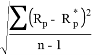 Â Â Â Â Â Â Â Â Â Â Â Â Â Â Â Â Â Â Â Â Â Â Â Â Â Â Â Â Â Â Â Â Â Â Â Â Â Â Â Â Â Â Â Â Â Â Â Â Â Â Â Â Â Â Â Â Â Â (3)
                                                          (3)
where Rp = Return of fund portfolio
         Rp*= Average return of fund portfolio
BETA
Beta co-efficient is a measure of systematic risk of the portfolio of each mutual fund scheme. It evaluates fund’s volatility as regard market index and measures the extent of co-movement of fund with that of market index. Beta (β) co-efficient can be calculated as –
β =                                                                 (4)
where COV(p.m)=Covariance between return of fund and market index.
            =Standard deviation of market index
COEFFICIENT OF VARIATION
reflects the degree to which the market and scheme returnsvary. A positive covariance means that the market and scheme returnsmove in the same direction whereas a negative covariance implies thatthe return moves in the opposite direction. Covariance is calculated usingthe formula:
C.V = (( / R p) Ã- 100)Â Â Â Â Â Â Â Â Â Â Â Â Â Â Â Â Â Â Â Â Â Â Â Â Â Â Â Â Â Â Â Â Â Â Â Â Â Â Â Â Â (5)
Rp is the mean return of the scheme
Coefficient of Correlation (r) measures the nature and the extent ofrelationship between stock market index return and the scheme’s returnfor a particular period. The co-movement of schemes performance withthat of market index is studied with the help of a simple linear regressionanalysis using the following formula:
 Â Â Â Â Â Â Â Â Â Â Â Â Â Â Â Â Â Â Â Â Â Â Â Â Â Â Â Â Â Â Â Â Â Â Â Â Â Â (6)
                                      (6)
Rmt = the return of market index
Rm*= Average return of market portfolio
COEFFICIENT OF DETERMINATION
Coefficient of determination (R2) indicates the extent to which the movement of fund can be explained by corresponding market index. It also a diversification index of fund portfolio. Higher the value of R2 (close to 1) indicates higher portfolio diversification and vice versa. Coefficient of Determinationis the square of the correlation co-efficient and indicates the degree of diversification.
SHARPE RATIO
Sharpe ratio (Si) is defined as –
  Si =                                                                   (7)
where Rp* = Average return of fund
         Rf = Risk free rate of return
           Standard deviation of return of the fund
TREYNOR’S INDEX
Treynor’s Index (Ti) is given by –
Ti = Â Â Â Â Â Â Â Â Â Â Â Â Â Â Â Â Â Â Â Â Â Â Â Â Â Â Â Â Â Â Â Â Â Â Â Â Â Â Â Â Â Â Â Â Â Â Â Â Â Â Â Â Â Â Â Â Â Â Â Â Â Â Â Â Â Â Â (8)
                                                                   (8)
 where Rp* = Average return of fund
          Rf = Risk free rate of return
              Sensitivity of fund return to market return
JENSEN’S ALPHA
Jensen’s alpha (α) is based on capital asset pricing model. Positive alpha indicates good performance. It is expressed as –
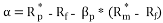 Â Â Â Â Â Â Â Â Â Â Â Â Â Â Â Â Â Â Â Â Â Â Â Â Â Â Â Â Â Â Â Â (9)
                                (9)
whereRp* = Average return of fund portfolio
         Rf = Risk free rate of return
           Sensitivity of fund return to market return
Rm*= Average return of market portfolio
FAMA’S MEASURE (FM)
Eugene Fama provides a framework to measure performance of the fund. Total return of a fund portfolio is divided into four components as- (1) risk free return (2) return from bearing systematic risk (3) compensation for inadequate diversification (4) return from fund selection. Net selectivity is the excess return adjusted for all risk. The fund manager can choose undervalued securities to earn greater return which is determined by the following formula –
 FM =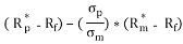 (10)
(10)
WhereRp* = Average return of fund portfolio
         Rf = Risk free rate of return
           = Standard deviation of portfolio return
 = Standard deviation of market index
         Rm*= Average return of market portfolio
Techniques of analysis
Stationary test
The stationary of the mutual fund return has been tested by Augmented Dickey Fuller test (1979) and Phillips Parron test(PP)(1988).
A more formal test that has become widely accepted is the unit root test. Let us consider the following model –
 Â Â Â Â Â Â Â Â Â Â Â Â Â Â (11)
              (11)
Where ut is the error term such that
E(ut)=0 for all t.
E(ut2)=σ2
E(utus)=0 t≠s
When Ï=1, we face a non stationary situation and conclude that Rt has a unit root. Therefore, to test if Rt is non stationary is to regress it on its one period lag value i.e. Rt-1. So the model rewrite as
 Â Â Â Â Â Â Â Â Â Â Â Â Â Â Â Â Â Â Â (12)
                   (12)
 Where δ= (Ï-1)
ut is a disturbance term with white noise.
Test the null hypothesis
H0: δ=0 (with alternative hypothesis H1:δ<0), then Ï=1 means that Rt has a unit root, and it is non stationary.
 We test statistical significance of
  .For this purpose we calculate the value of
  statistics as-
 (13)
Then compare the above statistical value with critical  values which have been initially tabulated by Augmented Dickey Fuller (ADF) using Monte Carlo experiments and subsequently extended by McKinnon (1991). If the absolute value statistics greater then absolute value of critical at our chosen level of significance, H0 is rejected and conclude that Rt series is stationary.
Phillips and Perron (1988) suggested an alternative nonparametric method of controlling for serial correlation when testing for the presence of unit root. The PP method estimates the non-augmented DF test equation and thus it is a generalization of ADF test procedure that allows for fairly mild assumptions concerning the distribution of errors. The PP regression equation is as follows:
 Â Â Â Â (14)
    (14)
The PP test corrects to the t statistic of the coefficient δ from the AR (1) regression to account for the serial correlation in ut. Here also the null hypothesis is H0: δ=0  [with alternative hypothesis H1:δ<0].
Three factor model
To test the explanatory power of historical risk on the present return of selected mutual funds schemes the following 3 factor model is used:
Rit – Rf = α0t+ α1tßi,t-1 + eit                               (15)
Rit – Rf = α0t+ α1tßi,t-1+α2tβ2i,t-1 + eit                 (16)
Rit – Rf = α0t+ α1tßi,t-1+α2tβ2i,t-1+α3tSi,t-1 + eit    (17)
Rit= return of ith fund at month t.
Rf= risk free rate of return.
ßi,t-1= historical systematic risk or beta of ith fund.
Si,t-1= historical residual risk or unsystematic risk of ith fund.
The present risk and return relationship measured by the following equation:
Rit – Rf = α0t+ α1tßit+α2tβ2it+α3tSit + eit             (18)
Rit= return of ith fund at month t.
Rf= risk free rate of return.
ßi= systematic risk or beta of ith fund.
Si= residual risk or unsystematic risk of ith fund.
Multicolinearity test
To detect multi co-linearity in the above regression equations Variance Inflation Factor (VIF) is used. In the presence of multi co-linearity the variance of the estimated c-efficient of kth explanatory variable is

When multi co-linearity is absent then Rk2=0 which is the squared multiple correlation between kth explanatory variable and other explanatory variables of the model.
The VIF is the ratio of two variances with multi co-linearity and without multi co-linearity. Thus,

 =1/1-Rk2Â Â Â Â Â Â Â (19)
The VIF values are calculated for each estimated slope co-efficient. From these values the variables are indentified which are responsible for multi co-linerity. By applying Rule Of Thumb it is concluded that when VIF≥10 that is R2k≥0.9 severe multi co-linearity exists for the kth explanatory variable.
Dummy variable regression model
To analyze the effect of recession(2008) on these selected mutual funds the following regression model is used –
 Â Â Â Â Â Â (20)
      (20)
j=1,2..20
Dt is the binary dummy variable (0 for 2005 – 2007 and 1 for 2009 – 2011)
St = Dt*(Rmt – Rft)
Rjt, Rmt, Rft are the return on mutual fund j, market return and Treasury gold bond rate respectively.
 measures the change in mean return between 2 sub-periods.
 measures the change in risk between 2 sub-periods.
Here each fund scheme mean return is regressed on market return.
Test for Heteroscedasticity:
In the past studies, the findings of heteroskedasticity in asset returns have been well documented. If the error variance is not constant, that is, heteroskedastic, then OLS estimation is inefficient. Moreover, the tendency in financial data for volatility clustering can be well captured in a framework of GARCH model. Therefore, we have modeled the time varying conditional variance in our study as a GARCH (Generalized Autoregressive Conditional Heteroscedastic) process.
But to be sure about whether GARCH type model is appropriate for the data or not, we have performed ARCH LM test (Engle 1982). This is a Lagrange Multiplier test for presence of ARCH effect in the residuals. For ARCH LM test we have first regressed return series on their one period lagged return series and have obtained the residuals ( ).The residuals then have been squared and regressed on their own lags for order one to four to test for ARCH effect. The estimated equation is:
 Â Â Â Â Â Â Â Â Â Â Â Â (21)
            (21)
We have then obtained the coefficient of determination ( ). The null hypothesis is that there is no ARCH error is
  . Under this null hypothesis the ARCH LM statistic is defined as TR2 where T represents the number of observations. LM statistic converges to a
  distribution. Hence we use this Lagrange Multiplier (LM) test for Autoregressive conditional heteroskedasticity (ARCH) to test the presence of heteroskedasticity in residual of the daily return series of seleted mutual fund schemes. If ARCH LM statistic is significant we confirm the presence of ARCH effect.
The autoregressive conditional heteroskedasticity (ARCH) model as developed by Engel (1982) is the extensively used time-series models in the finance related research. The ARCH (1) model suggests that the variance of residuals depends on the squared error terms from the past periods.
 Â Â Â Â Â Â Â Â Â Â Â Â Â Â Â Â Â Â Â (22)
                   (22)
The residual terms are conditionally normally distributed and serially uncorrelated.
GARCH Model
A generalization of this model is the GARCH specification. Bollerslev (1986) extended the ARCH model and it is based on the assumption that forecasts of time varying variance depend on the lagged variance of the variable under consideration. The GARCH specification is consistent with the return distribution of most financial assets, which is leptokurtic and it allows long memory in the variance of the conditional return distribution.
The simplest GARCH (1, 1) model can be written as-
Mean equation Rt = c +ut
Variance equation  Â Â Â (23)
   (23)
where αo > 0, α1 ≥ 0, α2 ≥ 0, and Rtis the return of the asset at time t, μ is the average return, and utis the residual return.
Since σ2 is current period variance based on past information, is called conditional variance. The conditional variance is a function of three terms: a constant term α0, squared error term in the previous period and the conditional variance of the previous period.
We use Akaike Information Criterion (AIC) to determine the order of GARCH model. Here ‘p‘ is the order of ARCH term and ‘q‘ is the order of GARCH term. We choose the order of ‘p‘ and ‘q‘ by the AIC criterion. Actually, we consider 5 as the maximum lag length and check the alternatives of GARCH model for selecting the appropriate one based on the AIC criterion. This will give us the best fitted GARCH model.
EGARCH MODEL
Nelson’s Exponential GARCH (1, 1) model can be written as-
 Â Â Â Â Â Â Â (24)
       (24)
The left hand side of equation 6 is the log of the conditional variance. This implies that the leverage effect is exponential and that the forecasts of the conditional variance are guaranteed to be non-negative. In this model, α1 is the GARCH term which indicates the impact of last period’s forecast variance. A positive α1 indicates volatility clustering means that positive return changes are accompanied with further positive changes and the other way around. β is the ARCH term which estimate the influence of news about volatility from the previous period on current period volatility. γ is the measure of leverage effect which indicate the differential reaction of volatility due to huge price increase or big price fall. The impact is not symmetric if γ ≠0. Ideally γ is expected to be negative implying that unfortunate condition has a larger influence on volatility than good condition of the same magnitude.
TGARCH model
This aspect of volatility modelling is captured by Threshold GRACH model developed independently by Glosten, Jaganathan, and Runkle (1993) and Zakoian (1994).
TGARCH (1, 1) model can be written as-
 Â Â Â Â Â Â Â Â Â Â Â Â Â Â Â Â Â Â Â Â Â Â Â Â Â Â Â Â Â Â Â Â Â (25)
                                 (25)
It-1 is the dummy variable indicates negative innovations. It-1 =1 if ut-1<0 and It-1 =1 if ut-1≥0.
Here good news means ut-1>0 and bad news means ut-1<0 have different effect on conditional variance. Good news has an influence on α1 and bad news has an impact on (α1+γ). If γ>0 then bad news increases volatility.
IGARCH model
R.F Engle and Tim Bollerslev (1986) proposed the Integrated GARCH model (IGARCH)which can capture the feature of “long memory” in financial time series i.e. the feature that a shock in the volatility series has impact on future volatility over a long horizon. In the model the persistent parameters sum up to one, and therefore there is a unit root in the GARCH process. The condition for this is α1+α2 =1. The equation of IGARCH model is-
 Â Â Â Â Â Â Â Â Â Â Â Â (26)
            (26)
PGARCH model
Z. Ding, C. W. Granger and R. F. Engle (1993) also developed a different variant of GARCH model named Power GARCH (PGARCH) model which is capable of capturing asymmetric response of volatility to positive and negative innovations. The PGARCH (1,1) modelspecifies  in the following form:
 Â Â Â Â Â Â Â Â Â (27)
         (27)
Where α1 and α2, are standard ARCH and GARCH parameters, γ denote the coefficient of
leverage effect and d is the parameter for the power term.