Multistage Heat Exchanger Design Optimization
Multistage Heat Exchanger Design Optimization using Sequential Quadratic Programming, Particle Swarm Optimization and Simulated Annealing methods
Islam Gusseinov[1], Cenker Aktemur[2], Dinara Kumasheva[3]
Department of Mechanical Engineering, Eastern Mediterranean University, via Mersin 10, Famagusta, N.Cyprus
ABSTRACT
    A multistage heat exchanger system is composed when it is requested to heat a single cold fluid stream with the aid of various existing hot streams. The present study concentrate on finding optimum area of three stages heat exchanger system which is connected in series. Optimum solution will be the smallest area permissible within given constraints, namely upper bounds and lower bounds. In general, this system is used to reach the required heat transfer between two fluids and get impressive heating or cooling of the fluid in one process. However, three heat exchangers connected in series will construct a huge system, which will require plenty of space to install. Another problem is the heat losses through the shell. Area of the heat exchangers increases, the heat losses will increase dramatically. That is why, we want to minimize the total of the heat transfer areas of the three exchangers by reaching the optimum solution for the efficiency.
Nomenclature
PSO=Particle Swarm Optimization
SA=Simulated Annealing
SQP=Sequential Quadratic Programming
HXÂ Â Â Â Â Â Â Â Â =Â Â Heat Exchanger
INPÂ Â Â Â Â Â Â Â =Â Â Inequality Constrained Nonlinear Program
QPÂ Â Â Â Â Â Â Â =Â Â Quadratic Programming
1. Introduction
A. Problem Description
    Many problems can be solved and optimized with the help of different kinds of software. One of the benchmark problems in applying various methods of optimization appears to be a Golinski’s speed reducer problem. There are many studies done on this topic, and many different types of methods like Simulated Annealing (SA), Sequential Quadratic programming (SQP), Genetic Algorithm (GA), and Particle Swarm Optimization (PSO) were carried out on Golinski’s problem. However, in this study, the same types of optimization methods will be applied on Three Stage Heat Exchanger problem, in order to find the optimal area, or in other words, the smallest area of three heat exchangers connected in series. In order to be able to perform optimization, Matlab software will be used which is a strong tool in optimization field, since it has wide range of optimization methods, prewritten by the developers. This allows us to directly use optimtools without re-writing codes again.
B. System Representation
    A fluid having a given flow rate W and specific heat Cp is heated from temperature To to T3 by passing three heat exchangers in series. In each heat exchanger (stage) the cold stream is heated with the aid of the hot fluid having the same flow rate W and specific heat Cp as the cold stream. The temperatures of the hot fluid entering the heat exchangers, t11, t21 and t31 and the overall heat transfer coefficients U1, U2, U3 of the exchangers are known constants. Drawing of the 3- Stage Heat Exchanger model is illustrated in Figure 1.


 Â Â Â Â Â Â Â Â Â Â Â T0T1T2T3
           T0T1T2T3


        t12t11     t22                                   t21   t32t31
Figure 1. Three Stage Heat Exchanger System [1]
C. Design Variables
Design parameters are the parameters which can be modified by designer in order to attain optimum solution and to satisfy all the constraints. Three stage heat exchanger involves eight design variables which are specified properly.
A1 – Area of the first HXÂ Â Â Â Â Â Â Â Â Â Â Â Â Â Â Â Â Â Â Â Â Â Â Â Â Â Â Â Â Â Â Â Â Â Â Â Â Â Â Â Â Â Â Â Â Â Â Â Â Â Â Â Â Â Â Â Â Â Â Â Â Â Â Â Â Â Â (x1)
A2 – Area of the second HXÂ Â Â Â Â Â Â Â Â Â Â Â Â Â Â Â Â Â Â Â Â Â Â Â Â Â Â Â Â Â Â Â Â Â Â Â Â Â Â Â Â Â Â Â Â Â Â Â Â Â Â Â Â Â (x2)
A3 – Area of the third HXÂ Â Â Â Â Â Â Â Â Â Â Â Â Â Â Â Â Â Â Â Â Â Â Â Â Â Â Â Â Â Â Â Â Â Â Â Â Â Â Â Â Â Â Â Â Â Â Â Â Â Â Â Â Â Â Â Â Â Â Â Â Â Â Â Â Â (x3)
T1 – Outlet temperature of first stage                                                 (x4)
T2 – Outlet temperature of second stage                                     (x5)
t12 – The temperature of the hot fluid entering first stage             (x6)
t22 – The temperatures of the hot fluid entering the second stage (x7)
t32 - The temperatures of the hot fluid entering the third stage               (x8)
Table 1: Design Variables [2]
|
Variable |
Symbol |
Units |
Lower Bound (LB) |
Upper Bound (UB) |
|
Area of the first stage |
A1 |
Sq.ft |
100 |
10000 |
|
Area of the second stage |
A2 |
Sq.ft |
1000 |
10000 |
|
Area of the third stage |
A3 |
Sq.ft |
1000 |
10000 |
|
Outlet temperature of first stage |
T1 |
OF |
10 |
1000 |
|
Outlet temperature of second stage |
T2 |
OF |
10 |
1000 |
|
The temperature of the hot fluid entering first stage |
t12 |
OF |
10 |
1000 |
|
The temperatures of the hot fluid entering the second stage |
t22 |
OF |
10 |
1000 |
|
The temperatures of the hot fluid entering the third stage |
t32 |
OF |
10 |
1000 |
The variable bounds for the problem are as follows [3]:
100 ≤ x1 ≤ 10000
1000 ≤ x2 ≤ 10000
1000 ≤ x3≤ 10000
10 ≤ x4≤ 1000
10 ≤ x5≤ 1000
10 ≤ x6≤ 1000
10 ≤ x7≤ 1000
10 ≤ x8≤ 1000
D. Design Constraints
    Design constraints can be of different types such as constraints related to physical properties, general constraints and constraints related to design variables, which are also called bounds. Constraints can be more flexible or inequality constraints and fixed which are called equality constraints. The main difference between equality and inequality constraints is the level of difficulty. Inequality constraint problems are easier to solve, since there is a chance to go from one limit to another, however equality constraints problem restricts the solution to one exact limit. In this particular case, there are six main constraints, eight bounds (constraints on design variables) and nine constraints within the bounds. That is why in Matlab just fifteen main constraints are used. The following table provides mathematical representation of six main constraints.
Table 2: Design Constraints
|
Constraint |
Symbol |
Units |
Limit |
|
|
G1 |
oF |
≤ 0 |
|
|
G2 |
oF |
≤ 0 |
|
|
G3 |
oF |
≤ 0 |
|
|
G4 |
Sq.ft |
≤ 0 |
|
|
G5 |
Sq.ft |
≤ 0 |
|
|
G6 |
Sq.ft |
≤ 0 |


E. Problem Formulation
    Previously the definition of optimization was given as the finding optimal solution to the problem by considering all design variables and satisfying all the constraints. Where the solution can be obtained by changing the design variables and initial, starting points for the optimizer. After choosing all the variables and establishing the constraints, it is time to formulate the objective function, which will give mathematical solution, by relating all needed design variables and constraints to each other. Objective function for this particular problem was formulated as it was described in work[5]. Objective function and constraints are provided below.
Objective function:Â Â Â Minimize 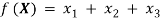
Subject to (constraints in right-hand column)
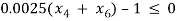 Â Â Â Â Â Â Â Â Â Â Â Â Â Â Â Â Â Â Â Â Â Â Â Â Â Â Â Â Â Â Â Â Â Â Â Â Â Â Â Â Â Â Â Â Â Â Â Â Â Â Â Â Â Â Â Â Â Â Â Â Â Â Â Â Â Â Â Â Â Â Â Â Â G1
                                                                         G1
 Â Â Â Â Â Â Â Â Â Â Â Â Â Â Â Â Â Â Â Â Â Â Â Â Â Â Â Â Â Â Â Â Â Â Â Â Â Â Â Â Â Â Â Â Â Â Â Â Â Â Â Â Â Â Â Â Â Â G2
                                                          G2
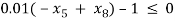 Â Â Â Â Â Â Â Â Â Â Â Â Â Â Â Â Â Â Â Â Â Â Â Â Â Â Â Â Â Â Â Â Â Â Â Â Â Â Â Â Â Â Â Â Â Â Â Â Â Â Â Â Â Â Â Â Â Â Â Â Â Â Â Â Â Â Â Â Â Â Â Â Â Â G3
                                                                          G3
 Â Â Â Â Â Â Â Â Â Â Â Â Â Â Â Â Â Â Â Â Â Â Â Â Â Â Â Â Â Â Â Â Â G4
                                 G4
 Â Â Â Â Â Â Â Â Â Â Â Â Â Â Â Â Â Â Â Â Â Â Â Â Â Â Â Â Â Â Â Â Â Â Â Â Â Â Â Â Â Â Â Â Â Â Â Â Â Â Â G5
                                                   G5
 Â Â Â Â Â Â Â Â Â Â Â Â Â Â Â Â Â Â Â Â Â Â Â Â Â Â Â Â Â Â Â Â Â Â Â Â Â Â Â Â Â Â Â Â Â Â Â G6
                                               G6
II. Results and Discussion
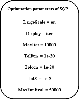
F. Sequential Quadratic Programming
Sequential Quadratic Programing (SQP) is one of the most popular methods in solving inequality constrained nonlinear program (INP). SQP appears to give reliable and effective results in short period of time. Within each iteration of SQP method Matlab solves quadratic programming (QP). This solution plays a guiding role for the next iteration [6]. Data from Matlab received for three stages HX is provided in table 3, down below.
Table 3: Optimization Results using SQP
|
Solution |
Units |
Run 1 |
Run 2 |
Run 3 |
|
x1 |
Sq.ft |
555.785990282356 |
368.842812105996 |
489.941608347603 |
|
x2 |
Sq.ft |
1496.77829557695 |
1409.78842135742 |
1475.12102289728 |
|
x3 |
Sq.ft |
5002.82363187765 |
5304.38006121906 |
5091.86834178931 |
|
x4 |
oF |
180.016508545819 |
161.355189743578 |
174.019885417799 |
|
x5 |
oF |
299.888637677655 |
287.834540297210 |
296.333509650773 |
|
x6 |
oF |
219.979103072183 |
238.629016924913 |
225.956135531385 |
|
x7 |
oF |
280.126421259455 |
273.511437056177 |
277.678961062453 |
|
x8 |
oF |
399.888245902272 |
387.832237792480 |
396.331510973503 |
|
G1 |
oF |
-1.09709549950265e-05 |
-3.95154181341839e-05 |
-5.99530482414679e-05 |
|
G2 |
oF |
-3.62402177345178e-06 |
-2.30289692231267e-05 |
-1.85404301938918e-05 |
|
G3 |
oF |
-3.85816583214904e-06 |
-2.30229861267750e-05 |
-1.99886687483053e-05 |
|
G4 |
Sq.ft |
-2.42690607324766 |
-3.12624794289877 |
-27.7786141939578 |
|
G5 |
Sq.ft |
-2.18310707871569 |
-17.3791291491361 |
-17.5780774553423 |
|
G6 |
Sq.ft |
-2.02720958227292 |
-12.1425335318781 |
-10.4304198068567 |
|
Objective |
Sq.ft |
7055.39 |
7083.01 |
7056.93 |
|
Optimizer parameters |
x0 = [550 1500 5000 200 300 200 300 400] |
x0 = [600 2000 6000 600 600 700 500 800] |
x0 = [300 1200 3000 450 550 650 450 600] |
* The violated Constraints are highlted in Bold


 Â Â Â Â Â Â Â Â Â Â Â Â Â Â Â Â Â Â Â Â Â Â Â Â Â Â Â Â Â Â Â NO
                               NO


 YES
YES
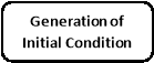
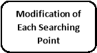
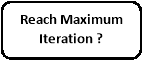
Figure 2. General Flow Chart and Optimization Parameters of SQP
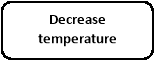
G. Simulated annealing
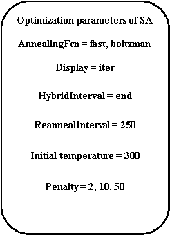
    Simulated annealing (SA) is a probabilistic method of optimization, used to find the global optimum point for given function. Moreover, it is a metaheuristic to locate global optimization in a large search space. It is mostly used for finding precise local minimum, while having a fixed time for all iterations. Simulated annealing could be considered as better option, rather than brute-force search or gradient descent.
    Simulated annealing takes its name from manufacturing process of slowly cooling the molten metal, in order to control the properties of the final product. In the same way, SQP slowly decreases the probability of getting bad result, by increasing the solution space [7].
    Using SA method provided different optimization result for the same inputs, constraints and design variables, than SQP method did. These results are tabulated in Table 4.
Table 4: Optimization Results using SA
|
Solution |
Units |
Run 1 |
Run 2 |
Run 3 |
|
x1 |
Sq.ft |
139.724828271076 |
100.000104807751 |
258,177990492450 |
|
x2 |
Sq.ft |
1000.64599816644 |
1017.44295810495 |
1000,00713464290 |
|
x3 |
Sq.ft |
1000.07536409596 |
4439.97459544385 |
3390,50971323642 |
|
x4 |
oF |
245.460108886459 |
91.8856667053922 |
365,912999644345 |
|
x5 |
oF |
388.784149405058 |
269.643483880431 |
374,204976990304 |
|
x6 |
oF |
971.698897292658 |
214.089384992577 |
958,928952825707 |
|
x7 |
oF |
490.653755999378 |
320.353186032579 |
483,076316148436 |
|
x8 |
oF |
752.433465643201 |
413.892877672396 |
472,961764726240 |
|
G1 |
oF |
2.02949239121487 |
-0.235063049022586 |
2,31205648350210 |
|
G2 |
oF |
0.243395435454855 |
0.245276619365850 |
0,228477155449455 |
|
G3 |
oF |
3.66459533266688 |
0.442499055677654 |
-0,0124603267437754 |
|
G4 |
Sq.ft |
-1.12564615524209 |
-1.81711694639683 |
-1.50580160468628 |
|
G5 |
Sq.ft |
-3.8020,6645185796 |
-1.02549103736873 |
-1.06820780542949 |
|
G6 |
Sq.ft |
-9.25189489858765 |
-6.45744633847843 |
-2.03521857259860 |
|
Objective |
Sq.ft |
2150.97 |
5564.30 |
4775.72 |
|
Optimizer parameters |
x0 = [300 1200 3000 450 550 650 450 600] Penalty = 2 |
x0 = [550 1500 5000 200 300 200 300 400] Penalty = 10 Boltzmann annealing Reannealing interval=250 |
x0= [600 2000 6000 600 600 700 500 800] Penalty = 50 Botzmann annealing Initial temp. = 300 |
* The violated Constraints are highlighted in Bold


 Â Â Â Â Â Â Â Â Â Â Â Â Â Â Â Â Â Â Â Â Â Â Â Â Â Â Â NO
                           NO


 NO
NO


YES
             YES


YES

Figure 3. General Flow Chart and Optimization Parameters of SA
H. Particle swarm optimization
    Particle Swarm Optimization (PSO) is a method of optimization that finds the optimum by repeatedly searching for the better solution, in comparison with the given value of the constraints and design variables. It solves a problem by sending the candidate solutions through the search space and letting them to find out the local optimum with respect to their mathematical algorithm. After finding local minimum these solutions are programed to compare their best point with the neighbouring one, that is how it is expected that the global optimum will be reached [8]. Based on the PSO method, the following results were retrieved.
Table 5: Optimization Results using PSO
|
Solution |
Units |
Run 1 |
Run 2 |
Run 3 |
|
x1 |
Sq.ft |
100.000049003836 |
100 |
100.000035217871 |
|
x2 |
Sq.ft |
1000.00011217875 |
1000 |
1000.00007680824 |
|
x3 |
Sq.ft |
1000 |
1000.00002296095 |
1000.00000062339 |
|
x4 |
oF |
121.418673285213 |
121.426230206343 |
121.427717593523 |
|
x5 |
oF |
460.000989443898 |
460.005701802001 |
460.000785308856 |
|
x6 |
oF |
278.507129110867 |
278.574674462544 |
278.563901342208 |
|
x7 |
oF |
544.648869935443 |
544.652837594674 |
544.644099603815 |
|
x8 |
oF |
560.000134288575 |
559.994330413195 |
559.999171302912 |
|
G1 |
oF |
-0.000263305653911416 |
9.94556734945640e-05 |
2.220804404479283 |
|
G2 |
oF |
1.20814848467031 |
1.20804826383677 |
1.20804602546329 |
|
G3 |
oF |
3.71887125054649 |
-0.000218022179330424 |
-1.93810245309178 |
|
G4 |
Sq.ft |
-6.80811877579254 |
7.03418059945398 |
-0.102022209626739 |
|
G5 |
Sq.ft |
-5.25140812853351 |
-13.9946636939421 |
-0.787525329855271 |
|
G6 |
Sq.ft |
-22.4404559549876 |
15.2219456185121 |
-1.06233827862889 |
|
Objective |
Sq.ft |
2112.081130937299 |
2160.404174693355 |
2220.804404479283 |
|
Optimizer parameters |
Swarm Size = 150 Penalty = 10 |
Swarm Size = 200 Â Â Â Â Â Â Â Â Â Â Â Â Â Penalty = 50 |
Swarm Size = 250 Â Â Â Penalty = 100 |
* The violated Constraints are highlted in Bold


YES
NO


Figure 4. General Flow Chart and Optimization Parameters of PSO
I. Comparison
After performing optimization on three stages HX system, using SQP, SA and PSO methods, the comparison table was constructed. It shows the time of optimization for each method, objective value received and function evaluation. As a result, we can see that the closest value for the area of the system is that of SQP method. This value is really close to the one, got by [1] after sixty iterations, which is 7049.
Table6: Comparison of Optimizers
|
Solution |
SQP |
SA |
PSO |
|
Objective Value |
7055.39 |
2150.97 |
2112.10 |
|
Function Evaluation |
382 |
17315 |
9600 |
|
Computation Time |
1.57 |
16.27 |
0.34 |
|
Ease of Implementation |
Difficult |
Medium |
Medium |
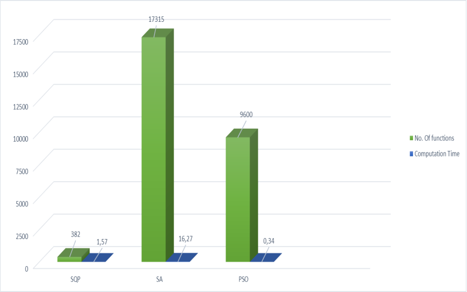
Figure 5. Computational cost vs NO. of functi
III. Conclusion
    Multistage system used for heat transfer is the topic of this case study. In more details, it is a three stages heat exchanger, where two fluids are exchanging the heat. The aim of this study was to calculate the minimum surface are of the system in such a way, that all of the requirements are fulfilled. In order to do so Matlab software was used, with its strong tools of optimization. There are many of tools in Matlab optimtool but we had chosen just three of them, in order to reach the optimum solution. These tools are SQP, SA and PSO, also called the methods of optimization. After performing optimization using each method separately with three runs for each, the results were obtained in the following manner. The weights for the three stages heat exchangers by all methods are: SQP = 7055.39 (Sq.ft), SA = 2150.97 (Sq.ft) and PSO = 2112.10 (Sq.ft). That is to show, that the closest value to the previous researches [1] was reached by SQP method, which is one of the best methods for finding optimum of INP problems. Also, SQP gave a result where no violation of constraints has occurred and that is one of the signs of good optimizer.
References
[1] M. AVRIEL and A. C. WILLIAMS, An Extension of Geometric Programming Engineering  Optimization, Journal of Engineering Mathematics, Vol. 5, No. 3, July 1971
[2] M. Avriel and D. J. Wilde, Engineering Design Under Uncertainty, Ind. Eng. Chem. Process Design and Dev.,8 (1969) 124-131.
[3] Singiresu S. RAO, Engineering Optimization: Theory and Practice. Fourth Edition, John Wiley & Sons, Inc., Hoboken, New Jersey
[4] A. H. Boas, Optimization via Linear and Dynamic Programming, Chem. Eng., 70 April 1, 1963, 85-88.
[5] L. T. Fan and C. S. Wang, The Discrete Maximum Principle, Wiley New York, 1964.
[6] Meredith J. Goldsmith,”Sequential Quadratic Programming Methods Based on Indefinite Hessian Approximation”, March 1999
[7] Retrieved from World Wide Web (Wikipedia), Jun 8, 2016
[8] Retrieved from World Wide Web (Wikipedia), Jun 8, 2016
Appendix
SQP
function NewFout = Heat_Exchanger_obj_sqp(x)
Fout = x(1)+x(2)+x(3);
function [c,ceq] =Heat_Exchanger_con_sqp(x)
ceq=0;
c = zeros(50,1);Â Â Â Â Â Â Â %Â Â Non-equality constraints
       c(1) = 0.0025*(x(4)+x(6)) – 1;
       c(2) = 0.0025*(-x(4)+x(5)+x(7)) – 1;
       c(3) = 0.01*(-x(5)+x(8)) – 1;
       c(4) = 100*x(1)-x(1)*x(6)+833.33252*x(4)-83333.333;
       c(5) = x(2)*x(4)-x(2)*x(7)-1250*x(4)+1250*x(5);
       c(6) = x(3)*x(5)-x(3)*x(8)-2500*x(5)+1250000;
      %Included just 6 constraints, since the rest are the bounds on
      %design variables
assignin(‘base’,’Constraint’,c);
clear all; close all; clc;
format short
tic
%% SQP
lb = [100Â Â Â 1000Â Â 1000Â Â Â 10Â Â 10Â Â 10Â Â 10Â 10];
ub = [10000Â 10000Â Â 10000Â Â Â 1000Â Â 1000Â Â 1000Â Â 1000Â 1000];
% x0 = [550 1500 5000 200 300 200 300 400] – RUN 1
% x0 = [600 2000 6000 600 600 700 500 800] – RUN 2
% x0 = [300 1200 3000 450 550 650 450 600] – RUN 3
Options = optimset(‘LargeScale’,’on’,’Display’,’iter’,’MaxIter’,10000,’TolFun’,1e-20,’Tolcon’,1e-20,’TolX’,1e-5,’MaxFunEval’,50000);
[X1,fval,exitflag,output]=fmincon(@Heat_Exchanger_obj_sqp,x0,[],[],[],[],lb,ub,@Heat_Exchanger_con_sqp,Options);
toc
PSO
function NewFout = Heat_Exchanger_obj_sqp(x)
Fout = x(1)+x(2)+x(3);
     ceq = zeros(50,1);          % Equality constraints
       c = zeros(50,1);          % Non-equality constraints
       c(1) = 0.0025*(x(4)+x(6)) – 1;
       c(2) = 0.0025*(-x(4)+x(5)+x(7)) – 1;
       c(3) = 0.01*(-x(5)+x(8)) – 1;
       c(4) = 100*x(1)-x(1)*x(6)+833.33252*x(4)-83333.333;
       c(5) = x(2)*x(4)-x(2)*x(7)-1250*x(4)+1250*x(5);
       c(6) = x(3)*x(5)-x(3)*x(8)-2500*x(5)+1250000;
      %Included just 6 constraints, since the rest are the bounds on
      %design variables
ceq = [];
SUM_OF_ALL_CONSTRAINT_VIOLATIONS = sum(c(find(c>0)));
assignin(‘base’,’cons’,c);
Penalty = 10;Â Â Â Â Â Â Â Â Â Â Â Â Â Â %Â Â try: 10, 50, 100
       if isempty(SUM_OF_ALL_CONSTRAINT_VIOLATIONS)
           NewFout = Fout;
       else
           NewFout = (Fout) + Penalty*SUM_OF_ALL_CONSTRAINT_VIOLATIONS;
       end
function [x,fval,exitflag,output] = pso(nvars,lb,ub)
tic
lb = [100Â Â Â 1000Â Â 1000Â Â Â 10Â Â 10Â Â 10Â Â 10Â 10];
ub = [10000Â 10000Â Â 10000Â Â Â 1000Â Â 1000Â Â 1000Â Â 1000Â 1000];
nvars=8;
% options = optimoptions (‘Display’, ‘iter’);
% Try 150,200,250 in each run
options = optimoptions (‘particleswarm’,’SwarmSize’,150);
[x,fval,exitflag,output]= particleswarm(@Heat_Exchanger_obj_sqp,nvars,lb,ub)
toc
SA
RUN 1
function [x,fval,exitflag,output] = sa(x0,lb,ub)
tic
%% This is an auto generated MATLAB file from Optimization Tool.
lb = [100Â Â Â 1000Â Â 1000Â Â Â 10Â Â 10Â Â 10Â Â 10Â 10];
ub = [10000Â 10000Â Â 10000Â Â Â 1000Â Â 1000Â Â 1000Â Â 1000Â 1000];
x0 = [300 1200 3000 450 550 650 450 600]
%% Start with the default options
options = optimoptions(‘simulannealbnd’);
%% Modify options setting
options = optimoptions(options,’Display’, ‘iter’);
options = optimoptions(options,’HybridInterval’, ‘end’);
[x,fval,exitflag,output] = simulannealbnd(@Heat_Exchanger_obj_sqp,x0,lb,ub,options);
toc
RUN 2
function [x,fval,exitflag,output] = sa1(x0,lb,ub,ReannealInterval_Data)
%% This is an auto generated MATLAB file from Optimization Tool.
lb = [100Â Â Â 1000Â Â 1000Â Â Â 10Â Â 10Â Â 10Â Â 10Â 10];
ub = [10000Â 10000Â Â 10000Â Â Â 1000Â Â 1000Â Â 1000Â Â 1000Â 1000];
x0 = [550 1500 5000 200 300 200 300 400]
%% Start with the default options
options = optimoptions(‘simulannealbnd’);
%% Modify options setting
options = optimoptions(options,’AnnealingFcn’, @annealingboltz);
options = optimoptions(options,’Display’, ‘iter’);
options = optimoptions(options,’HybridInterval’, ‘end’);
options = optimoptions(options,’ReannealInterval’, 250);
[x,fval,exitflag,output] = simulannealbnd(@Heat_Exchanger_obj_sqp,x0,lb,ub,options);
RUN 3
function [x,fval,exitflag,output] = sa2(x0,lb,ub,InitialTemperature_Data)
%% This is an auto generated MATLAB file from Optimization Tool.
lb = [100Â Â Â 1000Â Â 1000Â Â Â 10Â Â 10Â Â 10Â Â 10Â 10];
ub = [10000Â 10000Â Â 10000Â Â Â 1000Â Â 1000Â Â 1000Â Â 1000Â 1000];
x0 = [600 2000 6000 600 600 700 500 800]
%% Start with the default options
options = optimoptions(‘simulannealbnd’);