Performance Enhancement for Robot Localization

Performance Enhancement for Robot Localization and Fault Minimization Using Alternative Least Square Machine Learning Technique

ABSTRACT

Machine learning tools are used for specific applications. The purpose is to investigate proper machine learning tools for the SFU Mountain data-set. Impact: Revealing the appropriate machine learning tools will guide us to build a better data model. We are conducting semi-structured woodlands for fault diagnosis of how environmental variables affect the availability of important robotic services. Using a modeling framework, we are creating future scenarios of robotic service availability based upon local knowledge and climate projections. In addition, we are developing models derived from inputs to compare and potentially combine with local knowledge inputs. This allows us to assess, from several perspectives, how a critical component of community flexibility cans revolution in the future. Perfect productivities will be used to simplify deliberations in the groups on variation options that could minimize the negative consequences while seizing upon positive opportunities.

Keywords: Sfu-mountain, ALS, fault diagnosis etc.

I.INTRODUCTION

This paper considers the problem of recognizing locations based on their appearance. This problem has recently received attention in the context of large-scale global localization [Schindler et al., 2007] and loop-closure detection in mobile robotics [Ho and Newman, 2007]. We progresses the state of the art by developing a principled probabilistic framework for robotics algorithms for long-term deployment. Unlike many existing systems, our approach is not limited to localization we are able to decide if new observations originate from places already in the map, or rather from new, previously unseen places. This is possible even in environments where many places have similar sensory presence (a problem known as perceptual aliasing). Our system effectively learns a model of the common objects, which allows us to improve inference by reasoning about which sets of features are likely to appear or disappear. We present results which demonstrate that the system is capable of recognizing places while rejecting false matches due to perceptual aliasing even when such observations share many features. The approach also has reasonable computational cost fast enough for online loop closure detection in realistic mobile robotics difficulties where the plot covers numerous thousand places. We establish our scheme through identifying loop conclusions over a 4km path length in an initially-unknown outdoor environment, where the system detects a large fraction of the loop closures without false positives.

A calibrated sensor – If you have a sensor or instrument that is known to be accurate. It can be used to mark position interpretations for evaluation. Best laboratories will have devices that have been standardized beside and documentation including the specific reference alongside that they were regulated, as well as several improvement issues that need to be functional to the output.

B. Trail environment

Relatively few researchers have focused on the needs, trail location predilections, and involvements of the mountain biker. This research gives recreation supply managers with data that can prompt modification in the method they observe how trail environments should be managed. In one of the few comprehensive studies of mountain biker preferences for recreational settings and experiences, Cessford (1995) in a study for the Department of Conservation, New Zealand, measured altered users and their near of involvement about desired setting issues, trail types, trail conditions, downhill and uphill preferences, and social encounters. Major results presented that there was a relationship between biker preference and level of experience. For example, novice bikers preferred smooth, open, or clear trails and had low preference for obstacles and carrying bikes on sections not feasible for biking.

II. Literature survey

Jake Bruce, Jens Wawerla and Richard Vaughan [1] they have taken a dataset which are based on measured, coordinated and ground truth- aligned of woodland trail navigation in semi organized & shifting outdoor surroundings. The dataset is projected to support the growth of ground in robotics procedures for long-term arrangement in challenging outside situations. It takes total time more than 8 hours for trail navigation, with more accessible in the upcoming as the location variations. The data contain of interpretations from adjusted and coordinated sensors functioning at 5 Hz to 50 Hz in the form of color stereo and gray scale monocular camera images, perpendicular and push-broom laser scans, GPS sites, wheel odometry, inertial sizes, and atmospheric density standards.

Dudek & Jugessur [2] proposed an appearance-based navigation which is long history inside robotics; there has been substantial expansion in this field in last 5 years. Appearance-based navigation and loop closing recognition schemes working on routes on the instruction of a few kilometers in length are now common. Certainly, place detection schemes comparable in character to the one labeled here is now used equal in single-camera SLAM organizations intended for small scale uses in (Eade & Drummond, 2008) [3]. In real time application of these schemes on the scale of tens of kilometers or new has too initiated to be possible. For example, in (Milford & Wyeth, 2008) a scheme employing a set of naturally stimulated approaches accomplished effective loop closing recognition and plotting in an assembly of more than 12,000 images from a 66 km route, with processing time of less than 100 ms per image. The appearance-recognition element of the scheme was built on direct pattern matching, so scaled linearly with the size of the location. Working at a comparable scale, Bosse and Zlot define a place identic classification built on distinctive key points removed from 2-D lidar data (Bosse & Zlot, 2008) [5] and prove good precision-recall performance over an 18 km suburban data set.

Cummins & Newman, 2009 [6], they established loop closure recognition on a 1,000 km path, using a type of FAB-MAP which used to an inverted index structural design. One latest research is the improvement of combined schemes which syndicate appearance and metric data.

Olson [7] defined a method to increasing the robustness of overall loop closure detection schemes by using both appearance and comparative metric information to choose a single dependable set of loop closures from a bigger no. of applicants (Olson, 2008). The technique was assessed over numerous kilometers of urban data and shown to improve high precision loop closures even with the use of artificially poor image features. More loosely joined systems have also newly labeled in (Konolige et al., 2009; Newman et al., 2009). Significant applicable work also occurs on the more limited problem of overall localization.

II.PROBLEM STATEMENT

The data are highly challenging by virtue of the self-similarity of the natural terrain; the strong variations in lighting conditions, vegetation, weather, and traffic; and the three highly different trails. In contrast, we traverse challenging semi structured woodland trails, resulting in data useful for evaluating place recognition and mapping algorithms across changing conditions in natural terrain.

III. PROPOSED IMPLEMENTATION

Interestingly, optimizing the posterior probability therefore amounts to optimizing the likelihood function *plus* another term that depends only on the parameters. The posterior probability objective function turns out to be one of a class of so-called “penalized” likelihood functions where the likelihood is combined with mathematical functions of the parameters to create a new objective function.

Dataset

The SFU Mountain Dataset involves of numerous 100 GB of sensor data verified from Burnaby Mountain, British Columbia, Canada. Each traversal covers 4km of woodland trails with a 300m altitude change. Recordings contain complete video since 6 cameras, collection data from two LIDAR sensors, GPS, IMU and wheel encoders, plus calibration parameters for each sensor, and we provide the data in the form of ROS bag files, JPEG image files, and CSV text files. Jake Bruce, Jens Wawerla, and Richard Vaughan. The SFU Mountain Dataset: Semi-Structured Woodland Trails Under Changing Environmental Conditions,” in IEEE Int. Conf. on Robotics and Robotics, Factory on Visual Place Acknowledgment in Varying Surroundings. Seattle, USA, 2015.

Proposed Approach Flow

Alternating Least Square (ALS) Machine Learning

Alternating Least Squares starts by rotating between fixing one two coordinate for matrix dimension ui or vj that can be computed by solving the least-squares problem. This approach is handful as it improves the previous non-convex problem into a quadratic that can be solved easily [9]. A general description of the algorithm for ALS algorithm for collaborative filtering taken from Zhou et. al [11] is as follows:

Step 1: Initializing matrix V by allocating the average rating for that motion as the first row, and then for the small random numbers of the remaining entries.

The least squares simply adding up the squared differences between the model and the data.  Minimizing the sum of squared differences leads to the maximum likelihood estimates in many cases, but not always.  One good thing about least squares estimation is that it can be applied even when your model doesn’t actually conform to a probability distribution (or it’s very hard to write out or compute the probability distribution).One of the most important objective functions is the so-called posterior probability and the corresponding Maximum-Apostiori-Probability or MAP estimates/estimators. In contrast to ML estimation, MAP estimation says: “choose the parameters so the model is most probable given the data we observed.” Now the objective function is P(theta|X) and the equation to solve is

As you probably already guessed, the MAP and ML estimation problems are related via Bayes’ theorem, so that this can be written as

Once again, it is convenient to think about the optimization problem in log space, where the objective function breaks into three parts, only two of which actually depend on the parameters.

Step 2: Fix V, solve U by minimizing the RMSE function.

Step 3: Fix U, solve V by minimizing the MSE function similarly.

Step 4: Repeat Steps 2 and 3 until convergence.

Development tool

The raw data development kit provided on the

Autonomy Lab / SFU Mountain Dataset contains MATLAB demonstration code with file which gives further details.

Here, we will briefly discuss the most important features. Before running the scripts, steps are:

Step 1: Read curve’s points from the Excel file

Step 2: Extract Row Co-ordinate and column too

Step 3: Define fault rate

Step 4: fault Detected Parameter Machine// Compute current from voltage vector

Step 5: Do “coerce” to limit extrap values to positive values

Step 6: fault Detection rate minimization as per coverage distance

Step 7: Define sigmoid function regularization for numerical stability

Step 8: Define bernoulli probability weight matrix response update

Step 9:check convergence

Step 10: compute MSE

V.RESULT

In this section we present results showing sample trajectory matches, fault detection rate and MSE on results plots. The current implementation has ALS optimization built in, so compute scales linearly with the length of the dataset. For all experiments, computation was performed at real-time speed or faster on a standard Intel Core i7 PC.

We have evaluated our system with the public datasets from the [1] Project. The data were collected by a robotic platform in static and dynamic indoor, outdoor and mixed environments.

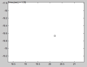
Figure 5.1: initial robot position in equilibrium state.

Above figure 5.1, the static position for robot 21.15 mm with 1.99-time slot fixing the pointer location having dynamic stages assign to each tracking region.

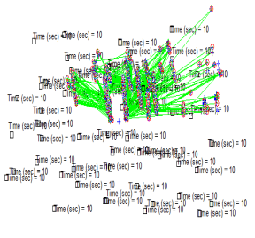
Figure 5.2: Robot define fix counter to each direction and tracking target position with dynamic localization in green lines.

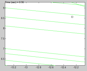
Figure 5.3: robot coverage distance divide region in track and make define position of laser range at 360^{o  ÂÂ} 

Above figure 5.3 specification the counter stage as per rotated angle and capture each laser to minimization and tolerate skipping factor from 6.5 -9 micro meter in 0.96 millisecond timing.

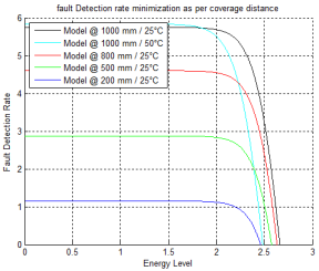
Figure 5.4: Fault detection rate minimization as per coverage distance over Energy level

Above figure 5.4, the model of 200 mm distance with weather circumstances at 25^oC having least fault detection rate i.e. 1.19, if we raise coverage or laser range of robot with same angle as previous weather circumstances meanwhile fault detection rate get highly maximized with same energy level or battery power of our robot configuration.

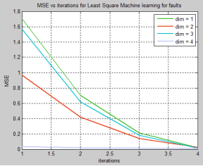
Figure 5.5: MSE vs iteration for least square machine learning for faults

Abovefigure 5.5, specification our proposed approach if raised no of dimension with same angular rotation of expert system means square error improving, hence minimum mean square error rate with 4- dimension of same iteration for our approach.

iteration	Fault minimization Rate
1	1.483500
2	1.034048
3	0.791479
4	0.340193
5	0.044917
6	0.000661
7	0.000000

The ALS method for computing correspondences, since they proved effective under several kinds of environments in the training datasets. In Fig. 5.5 we show the MSE curves obtained for our proposed simulation part which implemented in MATLAB tool with these parameters, we achieved a low MSE rate in the datasets with no false positives at dimension 4. In order to check the reliability of our algorithm with datasets, we used MATLAB as evaluation datasets. For these, we used our algorithm as a ALS, with the default configuration given above and the same vocabulary. This test shows that our method can work fine out of the box in many environments and situations, and that it is able to cope with sequences of images taken at low or high frequency, as long as they overlap.

VI.CONCLUSION

In this work, our proposed simulation of robot self-localization and utilizing all dimension and transferring position towards fix position by using a Alternate least square method. Our strategy is to create a visual experience for the library of raw visual images collected in different domains, to discover the appropiate visual patterns that clearly depicts the input scene, and use them for scene retrieval. In particular, we also showed that the appearance of the pose of the mined visual patterns, user laser range with tracking all coordinate with 360 degree which are matched with those of the database scenes by employing image-to-class distance and spatial pyramid matching. In future , the quadrate can be make for floor plan for learning object finder in internet of things and applying the deep learning into it.

REFERENCES

[1] Jake Bruce, Jens Wawerla and Richard Vaughan “The SFU Mountain Dataset: Semi-Structured Woodland Trails Under

Changing Environmental Conditions” Autonomy Lab, Simon Fraser University.

[2] Dudek, G. and Jugessur, D. Robust place recognition using local appearance based methods. In Proceedings of IEEE International Conference on Robotics and Automation, volume 2, 2000

[3] Eade, E. and Drummond, T. Unified loop closing and recovery for real time monocular slam. In Proc. 19th British Machine Vision Conference, 2008

[4] Milford, M.J. and Wyeth, G.F. Mapping a Suburb With a Single Camera Using a Biologically Inspired SLAM System. IEEE Transactions on Robotics, 24 (5):1038-1053, 2008.

[5] Bosse, M. and Zlot, R. Keypoint design and evaluation for place recognition in 2D lidar maps. In Robotics: Science and Systems Conference: Inside Data Association Workshop, 2008.

[6] Cummins, M. and Newman, P. Highly scalable

Appearance-only SLAM – FAB-MAP 2.0. In Pro-

ceedings of Robotics: Science and Systems, Seattle,

USA, June 2009.

[7] Olson, E. Robust and Efficient Robotic Mapping. PhD thesis, Massachusetts Institute of Technology, June 2008

[7] Konolige, K., Bowman, J., Chen, J.D., Mihelich, P., Calonder, M., Lepetit, V., and Fua, P. View-based maps. In Proceedings of Robotics: Science and Systems (RSS), 2009.

[8] Schindler, G., Brown, M., and Szeliski, R. City-Scale Location Recognition. In IEEE Conference on Computer Vision and Pattern Recognition, pp. 1-7, 2007

[9]Nist´er, D. and Stewenius, H. Scalable recognition with a vocabulary tree. In Conf. Computer Vision and Pattern Recognition, volume 2, pp. 2161-2168, 2006

[10] J´egou, H., Douze, M., and Schmid, C. Hamming embedding and weak geometric consistency for large scale image search. In David Forsyth, Philip Torr, Andrew Zisserman (ed.), European Conference on Computer Vision, volume I of LNCS, pp. 304-317. Springer, oct 2008.

[11] Y. Zhou, D. Wilkinson, R. Schreiber, and R. Pan. Large-scale parallel collaborative filtering for the netflix prize. In Proceedings of the 4th International Conference on Algorithmic Aspects in Information and Management, AAIM ’08, pages 337-348, Berlin, Heidelberg, 2008. Springer-Verlag.