Static Var Compensator to Improve Profile Voltage
Implementation of Static Var Compensator to Improve Profile Voltage On transmission System 70kV-150kV APJ Pasuruan
Abstract– System requirements for power is growing in line with the needs in line with population and industrial electricity consumption, so there is an alternative to maximize the utilization of the transmission line, one of them with equipment Flexible Alternating Current Transmission Systems (FACTS). Hardware FACTS device in this research one of which is a Static Var Compensator (SVC) to maintain the stability of the voltage remains constant at face value by injecting reactive power into the system can be controlled. Tool OCP contained in the software Electrical Transient Analysis Program (ETAP) is used to determine the location and capacity of SVC by applying the Genetic Algorithm (GA). To test the proposed method, the system standard IEEE 14-bus and the 70kV-150kV transmission system 12 bus APJ Pasuruan used for simulation in this study. From the analysis of 12 buses can be evidenced by the placement and capacity SVC in Bangil2 bus with a capacity of 43.2 MVAr Qc can raise the profile of the voltage to fall within the permitted margin of 0.95 p.u. to 1.05 p.u. Reviewed Bangil2 bus, bus Bulukandang, buses and bus Pandaan Sukorejo.serta can reduce the power of 10.158 MW and MVAr be 9.9966 45.048 44.660 MW and MVAr.
Index Terms– Static Var Compensator, Profile Voltage, ETAP Power Station, 70kV-150kV Transmission System.
I
N RECENT YEARS, the needs of the electric power system in Indonesia continues to increase along with the demand for electricity and the increase in population and industrial electricity consumption. In this case the development and construction of new plants and transmission lines are needed to meet the needs of the growing burden. Akantetapi it is determined based on the consideration of environmental and economic factors. In addition to the prohibitive cost, the construction of new transmission lines also require a very long time[1].So there is an alternative to maximize the utilization of transmission lines, one of which is by using equipment Flexible Alternating Current Transmission Systems (FACTS)[2].
FACTS devices of several types of devices, Static Var Compensator (SVC) is widely sudah digunakan around the
world, including in Indonesia itself has been applied in the GI Jember. Based on the standard PLN, the voltage value allowed on electric power system ranging from 0.95 to 1.05 pu of nominal voltage[3]..SVC Can maintain the stability of the voltage remains constant at a value nominalnya by injecting reactive power into the system can be controlled. Installation SVC at one point or some places could increase the value of the voltage profile and reduce power losses (losses)on the power system[4].
FACTS concept device was introduced by the Electric Power Research Institute (EPRI) in late 1980. Where the FACTS device can increase the capacity of the transmission system and control the flow of power (loadflow)is flexible[5].On the other hand FACTS devices can also reduce the cost of electrical energy generation and improve voltage stability of the transition state(transient)[6] [7].
Therefore, this paper will discuss the placement and the determination of optimal capacity SVC for voltage profile improvement 70-150 kV using Genetic Algorithms in the software ETAP Power Station
A. System Modeling Electricity
Modeling electric power system is defined as a network system consisting of components or electrical equipment such as generators, transformers, transmission line, and a load interconnected and establish a system.[8] [9]
B. Generator model
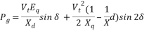
Generatorsare modeled as a PV bus. Which generator terminal voltage at a constant value. This is because the generator using AVR (AutomaticVoltageRegulator) to regulate the voltage on the bus. On the bus references (SlackBus), generator dioprasikan by rating voltage and phase angle const ant. In mathematical equations active power (MW) and reactive power (MVAr) generated by the generator can be written as follows:
 ………………………… (1)
   ………………………. (2)
Where:
Pg and Qg=Active and reactive power is delivered  terminal generator.
Vt = terminal voltage generator
δ = generator phase angle
Eq= internal voltage generator
Xd and Xq = synchronous reactance
C. Power Transformer
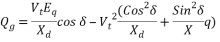
Power transformer of the power system can be expressed mathematically by the equation:
  …………………………………………………………….. (3)
  ………………………………………………… (4)
Where:
E = Voltage (pu)
F = frequency
N =Number of turns
 = maximum fluxsi
From the equation it can be seen that the mechanical power transformer primary and secondary winding is not connected, but electrically interconnected by electromagnetic induction.
D. Transmission Line
 Transmission lines are represented in accordance with the class of transmission. Representation of the transmission line based on the distance is divided into three parts, namely:
1. Short Transmission (l<80 km / 50 miles)
2. The transmission medium (80 km / 50 mi<l <240 km / 150 miles)
3. Transmission length (l> 240 km / 150 miles)

Figure 1. the equivalent circuit transmission line short

Figure 2. the equivalent circuit transmission line medium and length of
Short the transmission line, has a channel length of less than 80 km (50 miles) assumed that the capacitance value can be ignored and only the taking into account the value of the resistance (R) and inductive reactance (XL).With assumed in a balanced (balanced), the transmission line can show by using the equivalent circuit of the phase with resistance value (R) and inductive reactance (XL)which are connected in series (series impedance), which can be seen in Figure 2.1. While in the middle of the transmission line, the transmission line has a length of 80 km (50 miles) and 240 km (150 miles). In the middle of the transmission line, the capacitance conductor can not be ignored so that the conductor can be modeled using the equivalent circuit of one phase in the form of nominal À which can be seen in Figure 2.2. But for a long transmission line, capacitance and impedance conductive assumed contained on all the conductors to the limit of infinite.
E.  Electrical load
In power systems, there are two kinds of modeling the load is static load and dynamic load.
1) Model Static Load
Static load model is a model that represents active and reactive power as a function of the bus voltage and frequency. Static load in response to changes in voltage and frequency is reached quickly, so it tends to steady-state condition. Static load models are typically used for components such as resistive loads and lighting loads, and is also sometimes used to approach the dynamic components.
2) Model Load dynamic
Dynamic load model is a model that represents the active power and reactive follow the dynamics of the system variables, so that the condition can change at any time.
F. Drop Voltage
The Drop Voltage is the amount of voltage that is missing on a conductor. The voltage drop across the power line is generally proportional to the length of the channel and the load, and inversely proportional to the cross sectional area of the conductor. The magnitude of the voltage drop expressed either in percent or in the amount of Volt.
G. Static Var Compensator
Static Var Compensator or called SVC is one of the FACTS equipment Device consisting of a reactor component with a large set of inductive reactive power compensation and capacitor as a source of reactive power, power electronics equipment as well equipped as a switching device. Broadly speaking, the function of which is to preserve SVC (controller) voltage stability remain constant at its face value.
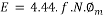
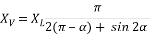
SVC is a generator / load connected shunt static VAR where output is set for the exchange of inductive or capacitive currents in order to maintain or control the power system can be varied. TCR (Thyristor Controlled Reactor) at the fundamental frequency can be treated as a variable inductance
   ………………………………………………. (5)
Where, XV is a variable reactance SVC while XL is the reactance caused by the fundamental frequency without control thyristor and α is the angle of ignition so that the total equivalent impedance of the controller can be expressed in:
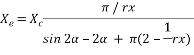  ……………………………………….. (6)
Value rx = XC / XL is given by the controller limit ignition angle limit of value fixed in accordance with the design. control law The steady state contained in the SVC typical VI characteristic figure 2.3 is
   …………………………………………………….. (7)
where V and I are rms voltage and current magnitude and Vref is the reference voltage. Typical values for slope XSL is 2 to 5%, tehadap SVC base; The value is necessary to avoid passing the limit of bus voltage variation is small. A typical value controlled voltage range  of Vref.[11] [12]
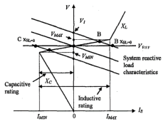
Figure 3. V I characteristics instate SVC steady
H. Power Flow method
By using the Newton Raphson method to analyze the power flow by forming a non-linear algebraic equations of power flow calculation can be determined by performing a comparison between the voltage change in voltage angle  and the magnitude of the voltage
  with active power changes
  and reactive power
  (k)).[11]In the mathematical equations of power flow can be written as follows:
 …………………………… (8)
Where:  is the value of active power (MW)
 is the value of reactive power (MVAr)
I. Software ETAP Power Station
ETAP (Electric Transient and Analysis Program)is a software full-graphics that can be used to design and test the condition of the existing electric power system. ETAP can be used to simulate the electrical power system offline in the form of a simulation module, monitoring the operation data in realtime, simulation, real time system optimization, energy management systems andsimulation of intelligent loads hedding. ETAP is designed to handle a variety of conditions and electric power system topologies both in the consumer side of the industry as well as to analyze the performance of the system at the utility. software Thisis equipped with facilities to support the simulation of such networks AC and DC (AC and DC networks),the design of cable networks, grid earth (groundgrid), GIS, panel design, arc-flash, coordination of protective devices (protective devices coordination /selectivity),and AC / DC control system diagram.
ETAP Power Station also provides a library that will simplify the design of an electrical system. library This can be edited or can be added to the information equipment. This software works by plant (project).Each plant must provide modeling support equipment associated with the analysis that will be performed. For instance generator, load data, channel data, etc. A plant consists of a sub-set of the electrical system that require special electrical components and interconnected. In Power Station, each plant must provide a data base for that purpose.
ETAP Power Station can be used to describe a single line diagram graphically and conduct some analysis / study of the Load Flow Short Circuit, the motor starting, harmonics, transient stability, protective device coordination, and Optimal Capacitor Placement.[13]
A few things to note in working with ETAP Power Station are:
- One Line Diagram, shows the relationship between the components / equipment so as to form an electrical system.
-  Library, information about all of the equipment that will be used in the electrical system. Data electrical and mechanical equipment details / full can simplify and improve the results of simulation / analysis.
- The standard is used, usually refers to the IEC or ANSI standards, the frequency of the system and method – the method used.
- Case Study, containing parameters – parameters related to the method of study to be performed and format of analytical results.
- Completeness of data from each element / component / electrical equipment on the system that will be very helpful analyzed the results of the simulation / analysis can approach the actual operational state.[13]
J. Genetic Algorithms on OCP tool within ETAP
Optimal Capacitor Placement (OCP) is one of the tools in the software ETAP Power Station which uses genetic algorithm for optimal capacitor placement. Genetic Algorithm is an optimization technique that is based on the theory of natural selection. An algorithm starts with the generation solutions with the diversity to represent the characteristics of the overall search space. By mutation and crossover characteristics that both have to be taken to the next generation. The optimal solution can be achieved through repeated generations. The most common method is based on a rule of thumb followed by running multiple power flow studies for fine tuning size and location. multiple power flow for fine tuning size and location.
K. Objective Function
The objective of the placement problems SVC is to improve the voltage profile and reduce the total power losses in power systems installed. The objective function is obtained from two terms. The first is the placement of SVC with the approach of the capacitor and the second is the total power loss. The objective function associated with the placement of the capacitor consists of a total power loss and the capacity of the capacitor. In general, the optimal capacitor placement and capacity can be written in the following equation [14]:
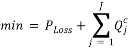    ……………….. ……. (9)
Subject to:
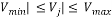  ……………………………….. (10)
  …………………………………….. (11)
Where:
P loss= Total power loss
J = Total Bus
 = Placement capacity capacitors on the bus j
Vj= voltage rms at bus j
V min= minimum voltage is allowed (pu)
V max= maximum voltage that allowed (pu)
 = maximum capacitor capacity permissible
 = minimum capacity capacitor bank
L. Operatinal Constraint
Along the feeder are required to remain within upper and lower limits after the addition of capasitors on the feeder. Voltage constrains can be taken into account by voltage.
M. Placement of Static Var Compensator
placement static var compensator used approach OCP. OCP is the optimal capacitor placement that exist in software ETAP power station which will be described in research methodology. Optimal placement of capacitors in the power system has many variables including the capacitor capacity, optimal placement, voltage and harmonics. Where in determining placement and optimum capacity, types of capacitors can be adjusted based on conditions on the ground. Namum considering these variables, making optimal placement becomes very complicated. So as to simplify the analysis, the type of capacitor can be assumed as follows:
1. The system is in equilibrium (balanced)
2. All types are considered constant load
N.  Capacitors Capacity
Capacitors In determining capacity, used capacity started based standard smallest capacity of capacitors and multiples thereof. So based on these standards, the capacity of the capacitor can be used as a discrete variable. and will be used as the capacity of the SVC.
In the analysis of the placement and the determination of the optimum capacity of capacitors to improve voltage profile and reduction in power losses, papers It uses the standard IEEE as a reference point in the implementation process and workmanship. Testing and research with survey data obtained from PT. PLN (Persero) APP TJBTB Probolinggo. With the data obtained, it can be simulated transmission system APJ Pasuruan 70 kV and 150 kV using software ETAP Power Station. Simulations can be done in the form of power flow or Load Flow, which is to know the profile of the voltage, active power, reactive power and losses that occur in the system 70 kV and 150 kV After conducting a study of power flow it is known conditions of the bus who suffered voltage drop (under voltage).If there are conditions that decrease the bus voltage below the allowable margin (0.95 <Vpu <1.05), it can be improved voltage profile by determining the optimal placement and capacity static var compensator (SVC) use the tool approaches OCP.[13]
A.  Flow studies
Flowused in the preparation of this study are as follows:
1) Start
2) Drawing single line diagrams.
3) Input data: data generator, a data channel, the data load.
   Running the simulation Load Flow using Method Newton Raphson
4) To check whether the voltage on the system is at the permitted margin of 0.95 ≤ V ≤ 1.05 pu
5) If “No”Perform simulation process OCP bus to get anywhere into optimal location for placement of the capacitor which is then replaced by the value of the capacitor SVC. Once the process OCP is complete, plug SVC finished.
6) Return to Step 4
7) If “Yes” go to step 8
8) Results and Analysis of the results
9) Done.
B. Flowchart
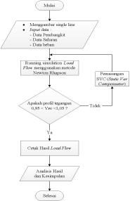
Figure 4. Flowchart solving
A. Modeling transmission system 70kV – 150kV APJ Pasuruan using software ETAP Power Station
Before running simulation modeling is required in advance PLN APJ Pasuruan sisitem transmission using software ETAP Power Station from pictures in the can when the survey. Modeling Single line diagramis done using software ETAP Power Station and to enter all of the data supports five image simulasi. Transmission system70kV -150kV APJ Pasuruan is still in the shade APP Probolinggo with 12 bus and were able to generate 632.4 MW power P and Q 391,92 MVar of PLTGU. Total peak load on the transmission system APJ Pasuruan P 327.75 129.8 MW Q MVar.
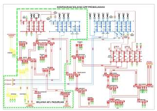
Source: PT PLN TJBTB APP Probolinggo
Figure 5. Single line diagram APP system probolinggo
B. Generating Data transmission line system 70kV – 150k APJ Pasuruan
Table 1. Data Capable of Generating Power transmission system 70kV – 150kV APJ Pasuruan
|
No. |
GENERATOR |
DATA SHEET APP PROBOLINGGO |
|
|
P (MW) |
Q (MVAr) |
||
|
1 |
PLTGU Grati 1 |
84.15 |
52 151 |
|
2 |
PLTGU Grati 1.1 |
127.5 |
79 017 |
|
3 |
PLTGU Grati 1.2 |
84.15 |
52 151 |
|
4 |
PLTGU Grati 1.3 |
84.15 |
52 151 |
|
5 |
PLTGU Grati 2.1 |
84.15 |
52 151 |
|
6 |
PLTGU Grati 2.2 |
84.15 |
52 151 |
|
7 |
PLTGU Grati 2.3 |
84.15 |
52 151 |
Source: PT PLN TJBTB APP Probolinggo
C. Load data transmission systems 70kV – 150kV APJ Pasuruan
Table 2. Data transmission system peak load of 70kV – 150kVAPJ Pasuruan
|
Line Transmission |
Transformer |
P (MW) |
Q (MVAr) |
|
GRATI |
Trafo1- 60 MVA |
12.6 |
3:22 |
|
BUMICOKRO |
Trafo1- 50 MVA |
39.15 |
11.82 |
|
Trafo2-60MVA |
46.8 |
16:12 |
|
|
GONDANGWETAN |
Trafo1-60MVA |
31.42 |
8:56 |
|
Trafo2-30MVA |
22:24 |
5.82 |
|
|
Trafo3-60MVA |
23:06 |
8:18 |
|
|
BANGIL1 |
Trafo1-60MVA |
27.26 |
6.94 |
|
Trafo1-20MVA |
16.74 |
6:04 |
|
|
REJOSO |
Trafo1-20MVA |
2.86 |
3:25 |
|
Trafo2-30MVA |
2:45 |
6 |
|
|
Trafo3-35 MVA |
8:21 |
2.1 |
|
|
PIER |
Trafo1-50MVA |
21.89 |
11:52 |
|
PANDAAN |
Trafo1-30MVA |
17:28 |
4.94 |
|
Trafo2-20MVA |
10.66 |
2.65 |
|
|
Trafo3-30MVA |
25.8 |
9.6 |
|
|
SUKOREJO |
Trafo1-30MVA |
17:42 |
6:06 |
|
BULUKANDANG |
Trafo1-60MVA |
24.4 |
6.93 |
|
Trafo2-20MVA |
8.66 |
2:44 |
|
|
PURWOSARI |
Trafo1 -60MVA |
13.85 |
7.61 |
Source: PT PLN TJBTB APP Probolinggo (peak load data)
D.  Line transmission data in system 70kV – 150kV APJ Pasuruan
Table 3. Line transmissiondata in system 70kV – 150kV Pasuruan
|
From |
To |
Circuit |
Distance (KM) |
Type Conductor |
|
GRATI |
GONDANGWETAN |
1 |
21.069 |
ACSR ZEBRA |
|
GRATI |
GONDANGWETAN |
2 |
21.069 |
ACSR ZEBRA |
|
GONDANG-WETAN |
BANGIL |
1 |
16.805 |
ACSR DOVE |
|
GONDANG-WETAN |
BANGIL |
2 |
16.805 |
ACSR DOVE |
|
BANGIL |
PANDAAN |
1 |
8,700 |
ACSR Ostrich |
|
BANGIL |
PANDAAN |
2 |
8,700 |
ACSR Ostrich |
|
BUMICO-KRO |
BANGIL |
1 |
6200 |
ACSR ZEBRA |
|
BANGIL |
SUKOREJO |
1 |
16,000 |
ACSR PIGEON |
|
BANGIL |
MOLDY-DANG |
1 |
24 770 |
ACSR DOVE |
|
BANGIL |
PIER |
1 |
6200 |
ACSR ZEBRA |
|
BANGIL |
PIER |
2 |
6200 |
ACSR ZEBRA |
|
GONDANG-WETAN |
PIER |
1 |
10 866 |
ACSR ZEBRA |
|
GONDANG-WETAN |
PIER |
2 |
10 866 |
ACSR ZEBRA |
|
PIER |
PURWOSA-RI |
1 |
22 422 |
ACSR ZEBRA |
|
PIER |
PURWOSA-RI |
2 |
22 422 |
ACSR ZEBRA |
|
GONDANG-WETAN |
REJOSO |
1 |
10 487 |
ACSR DOVE |
|
GONDANG-WETAN |
REJOSO |
2 |
10 487 |
ACSR DOVE |
Source: PT PLN TJBTB APP Probolinggo
E. Modelling single line transmission system diagram 70kV – 150kV APJ Pasuruan
Creating modeling a single line diagram70KV transmission systems – 150kV APJ Pasuruan on software ETAP Power Station is the first step in the analysis. Where in this modeling will be included all the data – technical data which includes capacity, generation, channel, transformer, step-up the transformer and the load.
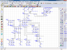
Figure 6 Modelling Single Line Diagram of the transmission system 70kV – 150kV APJ Pasuruan
F. Simulation Load Flow using Software ETAP Power Station on the conditions of the base case
Simulation load flow is intended to determine the initial condition of the system, determine the value of the voltage rating on every bus, knowing that the power in each channel and obtain the value of active and reactive power on the bus. Insimulation load flow thisusing methods Newthon Rhapson.
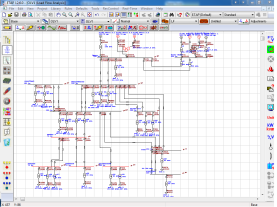
Figure 7. After the run with load flow in base case conditions.
Table 3. Profile voltage conditions of the base case
|
No. |
BUS ID |
V(pu) |
|
1. |
BANGIL 1 |
0.9568 |
|
2. |
BANGIL 2 |
0.9299 |
|
3. |
BULUKANDANG |
0.9497 |
|
4. |
BUMICOKRO |
0.9517 |
|
5. |
GRATI GITET |
0.1000 |
|
6. |
GONDANGWETAN |
0.9713 |
|
7. |
GRATI |
0.9992 |
|
8. |
PANDAAN |
0.9174 |
|
9. |
PIER |
0.9610 |
|
10. |
PURWOSARI |
0.9586 |
|
11. |
REJOSO SUMMIT |
0.9700 |
|
12. |
SUKOREJO |
0.9216 |
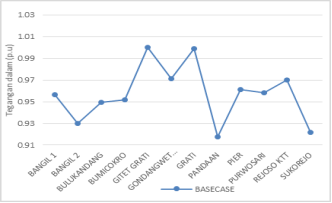
Figure 8. Graph voltage profile condition of base case
Based on the load flow inconditions basecase aboveand have been known to occur outside the voltage breach margin the permitted of 0.95 pu to 1 05 pu in Bangil2 bus, bus Bulu kandang, Pandaan bus, and the bus Sukorejo, it can be improved voltage profile by using analysis of Optimal Capacitor placement (OCP) for placement and capacity SVC.
G.  Placement Analysis SVC on 70kV-150kV transmission system APJ Pasuruan
In determining the placement and capacity SVC, this study uses Optimal Capacitor Placement (OCP) contained in software ETAP Power Station
1) Placement SVC using the OCP on software ETAP Power Station
Running OCP to find the location and capacity of the optimal capacitor will be applied in SVC using the techniques of Genetic Algorithm. By mutation and crossover characteristics that both have to be taken to the next generation. The optimal solution can be achieved through repeated generations. Before using OCP bus made the selection of candidates for the location of the installation of the capacitor dnature determine the location of SVC.
a) Determination Bus Candidates buses that will be placed capacitors
Click optimal capacitor placement

Figure 9 Tool in software ETAP Power Station
Determining bus candidate will have to be placed SVC uses pendektan of capacitors that bus who suffered critical contained in Table 3 in red. Buses were experiencing critical is Bangil2 bus, bus Pandaan, Sukorejo bus, bus Bulu kandang the voltage is under 0.95 puIn the simulation program OCP may be prescribed alone but should refer to the index of power losses bus candidate selection depends on the objectives to be achieved determination bus candidate is only done if there is voltage drop on the bus.
By the time the program will choose candidates to run OCP Bus provided in Table 3 are marked in red and will select the most optimal locations that will be placed along with the capacitor optimal capacitor capacity.
b) Determining the optimal location and capacity of the capacitor.
OCP will automatically calculate the minimum required capacitor capacity and optimal location to improve the voltage profile of the system. Which is then displayed on a single line diagram.
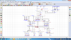
Figure 10. The location and capacity of the capacitor for the placement of SVC
After running the tool OCP on software ETAP PowerStation,the program displays the location and capacity of the optimal capacitor will be installed on buses that have been determined.
c)  The location and capacity of the capacitor
By using the tools OCPon software ETAPcapacitor placement can be optimized with the right to correct the voltage rating by bus candidate. The results of the OCP is:
Table 4 Result determination of SVC with OCP
|
Results OCP |
||||
|
ID Bus |
Banks (kVar) |
kV |
Number Of Banks |
Total Banks (Kvar) |
|
BANGIL2 |
10 800 |
70 |
4 |
43 200 |
After adding the candidate buses that have a voltage drop outside the limits of ± 5% (standard tolerance AC voltage PLN) found the number and location of capacitors that are in the bus as it exists in table 4.after obtaining the location and capacity of the OCP, her location is located on theBangil2 bus banks (kVar) 10800 multiplied by four (the number of banks)then the result 43200 kVar or in a larger unit Qc its 43.2 MVAr SVC is entered as the capacity to improve the voltage profile. After that run back with a loadflow to ensure the voltage profile are at the margin set.

Figure 11 is run back to the loadflow after placement on the Bus Bangil2 SVC.
From the results of simulation loadflowstelah SVC installation can be in the know that the profile of the voltage on the bus who suffered undervoltage returns to normal.
Table 5. Profile voltage before and after the installation of SVC
|
ID bus |
Basecase (pu) |
SVC (pu) |
|
BANGIL1 |
0.9612 |
0.9568 |
|
BANGIL 2 |
0.9299 |
0.9644 |
|
BULUKANDANG |
0.9540 |
0.9497 |
|
BUMICOKRO |
0.9561 |
0.9517 |
|
GITET GRATI |
1.000 |
1.0000 |
|
GONDANGWETAN |
0.9745 |
0.9713 |
|
GRATI |
0.9992 |
0.9992 |
|
PANDAAN |
0.9514 |
0.9174 |
|
PIER |
0.9610 |
0.9650 |
|
PURWOSARI |
0.9625 |
0.9586 |
|
REJOSO |
0.97 |
0.9732 |
|
SUKOREJO |
0.9558 |
0.9216 |
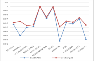
Figure 12. Comparison of the voltage profile (pu) before and after the installation of
Table 6. Loss of active power loss (Ploss) on the channel before and after the installation of SVC
|
channel |
Basecase (MW) |
SVC (MW) |
|
bmckro-bngil1 |
0181 |
0183 |
|
bmckro-bngil2 |
0181 |
0183 |
|
bngil1-blkdng |
0188 |
0190 |
|
bngil1-pier1 |
0158 |
0153 |
|
bngil1-pier2 |
0158 |
0153 |
|
bngil2-pdaan1 |
0230 |
0261 |
|
bngil2-pdaan2 |
0230 |
0261 |
|
bngil2-skj1 |
0052 |
0057 |
|
bngil2-skj2 |
0052 |
0057 |
|
gdwtan-bngil11 |
0682 |
0655 |
|
gdwtan-bngil12 |
0682 |
0655 |
|
gdwtan-pier1 |
0528 |
0507 |
|
gdwtan-pier2 |
0528 |
0507 |
|
gdwtan-rjso1 |
0008 |
0008 |
|
gdwtan-rjso2 |
0008 |
0008 |
|
grti-gdwtan1 |
2,155 |
2,089 |
|
grti-gdwtan2 |
2,155 |
2,089 |
|
prwsri1 |
0.013 |
0.013 |
|
pier-pier-prwsri2 |
0.013 |
0.013 |
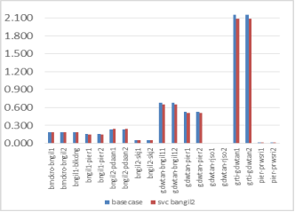
Figure 13. Comparison of active power losses (Ploss) before and after installation of SVC
Table 7. loss reactive power(Qloss) on the channel before and after the installation of SVC
|
channel |
Basecase (MW) |
SVC (MW) |
|
bmckro-bngil1 |
0117 |
0118 |
|
bmckro-bngil2 |
0117 |
0118 |
|
bngil1-blkdng |
0166 |
0167 |
|
bngil1-pier1 |
0168 |
0161 |
|
bngil1-pier2 |
0168 |
0161 |
|
bngil2-pdaan1 |
0294 |
0316 |
|
bngil2-pdaan2 |
0294 |
0316 |
|
bngil2-skj1 |
0.056 |
0.060 |
|
bngil2-skj2 |
0.056 |
0.060 |
|
gdwtan-bngil11 |
0723 |
0693 |
|
gdwtan-bngil12 |
0723 |
0693 |
|
gdwtan-pier1 |
0560 |
0537 |
|
gdwtan-pier2 |
0560 |
0537 |
|
gdwtan-rjso1 |
0008 |
0008 |
|
gdwtan-rjso2 |
0008 |
0008 |
|
grti-gdwtan1 |
7223 |
6995 |
|
grti-gdwtan2 |
7223 |
6995 |
|
prwsri1 |
0.014 |
0.014 |
|
pier-pier-prwsri2 |
0.014 |
0.014 |
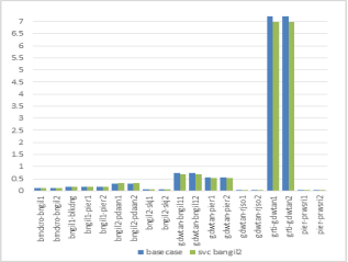
Figure 14. Loss loss reactive power (Qloss) on the channel before and after the installation of SVC
Table 8. Comparison of Ploss and Qlossconditions basecase and after the installation of SVC
|
Total Ploss(MW) and Qloss (MVAr) |
MW |
MVAr |
|
basecase |
10.158 |
45.048 |
|
With SVC |
9.966 |
44.660 |
Installation SVC Bangil2 bus with a capacity of 43.2 MV Ar Qc, is able to reduce losses of active power losses overall 10.158 MW to 9.966 MW and loss reactive power losses total of 45.048 MV Ar be 44.660 MV Ar because of SVC reactive power compensation so that voltage profile awake and keep working on the authorized limit.
-   After the run using the tool Optimal Capacitor Placement (OCP) to determine the location and capacity of SVC, bus chosen to put SVC is on Bangil2 bus with a capacity of 43.2 MVAr Qc.
-  Once installed SVC at bus that has been determined by the OCP bus voltage profile on Bangil2 of 0.9299 pu pu be 0.9644, from 0.9497 Bulukandang bus into 0.9540 pu pu, Bus Pandaan of 0.9174 pu pu be 0.9514, and the bus Sukorejo of 0.9216 pu pu be 0.9558, which previously suffered critical back on limits / margins allowed (0.95 pu <1.05 pu)
-  While the loss of power loss can be reduced while the loss of active power loss(Ploss) which can be reduced from 10.158 MW to 9.966 MW and reactive power losses(Q</e